- Original Paper
- Open access
- Published:
An energy concept for macroscopic traffic flow modelling
European Transport Research Review volume 4, pages 57–66 (2012)
Abstract
Introduction The main differences between the deterministic macroscopic models are to be found in pressure expressions and representation of various phases observed experimentally.
Methods In this paper, using the laws of fluid dynamics and thermodynamics to describe the traffic flow reality, a new expression of pressure is made and a second order model is proposed.
Results It represents different traffic flow phases and, thus, conditions for transition between phases become clear. In addition, our approach suggests solutions to a number of problems yet to be resolved. Afterwards, simulations are presented which show some agreement with experimental data.
Conclusion Finally, the proposed model highlights different types of possible actions for traffic flow control.
1 Introduction
One of the widely used approaches for traffic flow modelling is the macroscopic one in which the traffic is considered as a particular continuous flow treated as an atypical ideal fluid. In this case, we are interested in the spatial and temporal evolution of the main state variables ρ(x, t) and v(x, t), which respectively represent density and speed of cars located in point x at time t on road. So the main objective here is to propose models that can reproduce dynamic behaviours, such as free flow, congested flow, synchronized flow, and so on.
The work presented in this paper is based on physical laws which we adapt to the reality and the particularity of traffic flow in order to obtain a realistic dynamic model. Indeed, the traffic flow is a physical system in which it is not easy to distinguish between intrinsic behaviour effect and external actions. This distinction is necessary to study the stability and control problems of traffic flow. It would be thus desirable to obtain a model as realistic as possible for simulation, allowing us to highlight the possible actions and to develop efficient algorithms for traffic flow control.
The paper is organized as follows. In Section 2 we review the main macroscopic models. The results obtained are presented in the next three sections. Section 3 describes the principles of the proposed approach. Based on these principles we build, in Sections 4 and 5, a macroscopic traffic flow model and its variants. Finally, we present in Section 6 a numerical scheme used in our case, and we conclude with some simulations.
2 Macroscopic traffic flow modelling
The modelling studies of traffic flow started in the thirties. Greenshields [11] proposed an algebraic relationship between the traffic speed and the traffic density.

where νmax and ρmax represent, the maximal speed and the maximal density, respectively.
Thereafter, Lighthill and Whitham [17] and Richards [28] proposed the first macroscopic model, called the LWR model. However, this model does not represent the whole diversity of traffic flow dynamics. The first second order model was proposed by Payne [26] and Whitham [29] in terms of state variables; speed and density. This model, called the PW model, was criticized by Daganzo [8] for, notably, its lack of physical sense. Thereafter, Aw and Rascle [2], Colombo [4], Helbing [13], Zhang [31] and Lebacque et al. [16] proposed models to remedy the deficiency of the (LWR) model as well as the shortcomings and contradictions of the (PW) model.
Otherwise, Kerner [15] has been working on traffic understanding and he has brought in the concept of “Three-phase traffic theory”. Indeed, on the basis of experimental studies, Kerner proposed three-phases: Free flow, wide moving jams and Synchronized flow. Colombo and Goatin, as for them, compared Kerner experimental with fundamental diagram and suggested that a good model must show two qualitatively different behaviours (i.e. phases) [5–7].
3 Model design
Let us recall that all deterministic macroscopic models are based on analogy with ideal fluid flow. We must note that the first significant adaptation resides on the use of particle derivative [2], which provides an anisotropic character to traffic flow. This ensures that information propagation speed remains less than, or equal to, traffic flow speed. Currently, the main differences appear at the level of:
-
Taking into account “multiphasic” hybrid aspect of traffic flow
-
Choosing the pressure expression according to density
Generally, the proposed expressions for pressure emanate from field of thermodynamics [1, 2, 19]. In the approach presented here, we propose to deduce pressure expression from that of internal energy “potential” [21]. Thus, we shall consider the energy concept as the starting point of the traffic flow modelling. Indeed, it may be helpful to highlight the existence of several dynamics for traffic flow and to determine the pressure expression necessary to use from the analogy with fluid flow. Of course, the expression of this energy must take into account the specificity of the traffic. Furthermore, the model must respect the quasi-totality of the conditions (mentioned in [2, 4, 15]) to be physically valid. Moreover, it has to show that coming back to the free flow phase of vehicles at downstream front of jam must be done intrinsically (without exogenous action).
The model presented below is based on two assumptions.
-
Elasticity principle is applicable
-
There is an internal energy “potential”.
The first will take into account this singularity observed experimentally, namely the existence of several phases in traffic flow. The second will allow us to determine the pressure expression according to density and road characteristics.
3.1 Elasticity principle
A system is said to be elastic when it goes back to its steady state after the disappearance of stress. The stress can be of compression or expansion type and its effect is stored in internal energy “potential” form.
Thus, with the disappearance of stress, a force, created by this potential, brings the system back to its steady state.
In the traffic case, when, for some reason, drivers decelerate, they approach more and more to the vehicles that precede them, which increases the density with regard to the critical density. This situation stays unchanged as long as the stress remains and we can say that the system is in a metastable state. As soon as this stress vanishes, the drivers, quite natural, accelerate to reach their cruising speed (ν c ) which corresponds to critical density (ρ c ). We have, therefore, the emergence of an internal energy “potential” that compensates, in this case, the loss of kinetic energy. However, when traffic density becomes lower than the critical density, drivers will not seek to return to the critical density without external action. In other words, they can travel freely (while respecting the limit speed naturally !). We can, therefore, say that, in the traffic case, only decompression force must be taken into account. The model should, therefore, allow this return to steady state intrinsically. Thus, we should consider elasticity phenomenon for the decompression case only (i.e. ρ > ρ c ).
3.2 Internal energy density and pressure
3.2.1 Pressure expression
Again, the reasoning is based on some analogies with perfect fluid flow. So, we can consider that the internal energy “potential” is stored in terms of pressure and temperature [20], but only according to pressure for traffic flow. To find the expression of this pressure, we consider the first law of thermodynamics for a reversible process

where U, V, T and S represent respectively the internal energy, volume, temperature and entropy. Moreover, as the traffic flow is seen as an isentropic fluid, we have dS = 0 and dU = − pdV. Besides, we get the energy density from the relationship U = εV. The total differential gives

and hence

The pressure expression depends on that which will be given to internal energy density ε. In other respects, we can express this density as a function of ρ.
For this, we can use the following phenomenological expression: [30] in [27]

where ε(ρ) represents the density of internal energy of the traffic flow which should vanish for steady state (ρ = ρ c ). The first term in Eq. 5 is responsible for the sound wave, where c is the equivalent of sound speed in medium. The second term is responsible for the dispersion of this wave. Afterwards, we will keep only the first term in Eq. 5:

To comply with the first assumption, the internal energy will be considered only in the congested traffic flow case (ie only when ρ c < ρ ≤ ρmax) which ensures, at the same time, uniform property to ε(ρ).
We have to develop Eq. 4 to obtain the closure equation linking p to ρ. We know, on the one hand, that the volume is equal to the inverse of the density. On the other hand, according to the first assumption, the internal energy has sense only for ρ c < ρ < ρmax and it depends on the deviation from ρ c . It is the same for volume V, which makes sense only for ρ > ρ c . So, we consider the difference (ρ − ρ c ) as the inverse of volume V:

and rewriting Eq. 4 we have

Making the necessary replacements, we obtain the closure equation

We will use this expression during model building instead of the pressure of a PW model [14, 26],

Were V e (ρ) and TPW represent equilibrium speed and reaction time.
3.2.2 Multiphasic traffic flow concept
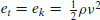
We will use the concept of total energy to highlight multiphasic aspect of traffic flow. Indeed, total energy (considered as the Hamiltonian) [20] provides the number of algebraically independent variables (state variables), necessary and sufficient, for system dynamic representation. The others are deduced as closure equations. Therefore, to obtain the total energy, we will take the following expression as kinetic energy density:

Then, the total energy density is written as

This expression shows that we have two terms corresponding to two forms of energy storage and, thus, at the most, two state variables, namely, ρ and v.
We can already distinguish the following cases:
-
ρ ≤ ρ c
There is no constraint on the traffic flow here, so the internal energy vanishes. The expression of the density of the total energy is reduced to
 , ie we have only one form of energy storage and, thus, one state variable. Then, ρ and ν are linked algebraically.
 -
ρ c < ρ ≤ ρmax
In this case, we should consider the total energy density given by Eq. 12. This corresponds to the presence of both forms of energy, which implies the presence of two state variables.
 , ie we have only one form of energy storage and, thus, one state variable. Then, ρ and ν are linked algebraically.
We will have only one evolution equation in the first case and two in the second. Thereafter, we distinguish several possible scenarios depending on the value of the density. Each one represents a particular phase of traffic flow:
-
Free flow (ρ ≤ ρ c )
-
Congested flow (ρ c < ρ < ρmax)
-
Congested and saturated flow (ρ = ρmax).
4 Proposed expression
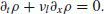
Naturally, the first equation to take into account is the equation describing the vehicles conservation:

The second model equation is based on Newton’s law. However, in order to take into account traffic flow anisotropy, as [2, 4] and [31], we express the acceleration according to particle derivative of pressure. So, we consider the following expression:

In order to have an easy model to use, we consider that acceleration is proportional to  ; then we must replace variable ν by a constant and take ν = ν
c
. This choice allows us to have q
c
as the road characteristic. We can then write
; then we must replace variable ν by a constant and take ν = ν
c
. This choice allows us to have q
c
as the road characteristic. We can then write

Note that this expression, without the constant, is similar to the initial form of the AR model [2].
By replacing pressure p with its expression (6), we obtain

and the speed evolution equation can be written as

We put this expression into the following form:

We obtain, then, the first expression of the speed evolution equation:

Substituting c by the expression (see Appendix), we get the model equations

or in matrix form:

with 
Remark
-
The model depends explicitly on characteristic parameters of the considered road (ρ c , ν c and ρmax).
-
The corresponding eigenvalues of this matrix are
 .
. -
The system Eq. 21 is strictly hyperbolic for ρ > ρ c .
-
As
 the wave velocities do not exceed the traffic flow speed.
 .
. the wave velocities do not exceed the traffic flow speed.
5 Various phases of the traffic flow
5.1 Free flow phase (ρ ≤ ρ c )
According to the first assumption in Section 3, the internal energy is nil. It remains the kinetic energy which depends on the density and speed. Knowing that state variables are those that appear in the energy expression, we notice that either ρ or ν can play the role of state variable. Since state variables must be linked algebraically, we take the vehicle conservation equation as the evolution one and consider, as algebraic relationship, a modified expression of the linear relationship (1):

This modification allows us to take into account the fact that the relationship is valid only for (ρ ≤ ρ c ).
Remark
The free flow case corresponds to the vanishing of pressure forces. Therefore, the acceleration expression is reduced to  . In other words, we have the Burgers’ equation. This confirms the fact that we have only one evolution equation.
We examine below the behaviours for which the value of the density becomes, in same way or another, lower than that of the critical density. We suggest classifying these dynamics in three main phases.
5.2 Congested phase and forced regime (ρ c < ρ < ρmax)
This phase represents the phenomenon known as “moving jams”. In this phase, we will distinguish behaviour within the congestion from which occurs upstream. Note that the origin derives from density and/or speed deteriorations.
5.2.1 Speed deterioration effects
-
Evolution at upstream of congestion
This case corresponds to the presence of a cluster forced to drive at a speed determined by a given vehicle, a leader. For instance, the presence of a truck, travelling at a speed lower than the critical one, compels the following vehicles to drive at its speed. Then, a cluster is formed which moves at a speed ν l (t, x) < ν c . We have, therefore, the appearance of an internal energy which compensates for the reduction of the kinetic one. Note that the speed of the leader represents exogenous distributed action. This corresponds to a forced regime for a dynamic system and to take it into account, we add a second member to the second equation of the system (20):
 (23)
(23)where ν l (x, t) and τ l represent, respectively, the leader speed and a time constant.
-
Evolution inside congestion
When the situation persists, the traffic flow tends towards a metastable state, mentioned by Kerner [15]. In the particular case when the leader speed is constant and the situation continues, a stationary regime establishes at ν = ν l . Then a cluster is formed, moving with constant speed. Note that this case represents the so-called moving jam phenomenon for low ν l (x, t) values.
To get the corresponding particular model, we rewrite the system (23) with ν = ν l . We, therefore, obtain a single equation that characterizes the cluster that moves at a constant speed:
 (24)
(24)In other words,we have a convective equation with constant speed fixed by the leader. In contrast to the free flow case, we do not have here an algebraic relationship between ρ and ν l .


5.2.2 Density deterioration effects (bottleneck)
Several problems can cause a narrowing of the roadway, for instance:
-
(a)
presence of a large number of trucks that take up a lane over a great distance.
-
(b)
motorway services can reduce the number of available lanes to users to ensure road maintenance.
-
(c)
accidents, as well as incidents of various kinds, compel rescue services and/or authorities to close lane.
In this case, we can divide the considered section of the road into two zones where the characteristics are ρcbo, νcbo and ρmaxbo within the congestion and ρ c , ν c and ρmax upstream of the congestion.
-
Evolution inside congestion
The equations to be used in this case have to reflect the temporary characteristics of the concerned zone. Indeed, the maximum density is reduced, the reduction ratio depending on the narrowing rate of the road. We should also change the values of the critical density and critical speed that must be adapted into the area. The model then takes the form
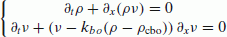 (25)
(25)where
 .
.Note that the zone concerned can move (case a) or be fixed (cases b and c).
-
Evolution at upstream of congestion
Upstream of the congestion, vehicles must slow down to adapt their speed to that imposed by the density of jam zone. This corresponds to the case of the “follow-the-leader” seen above, but, here, the leader is fictitious.
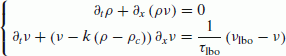 (26)
(26)The leader speed νlbo ≤ νcbo and it depends on density values within, and upstream of, the congestion.

 .
.
5.3 Congested and saturated phase (ρ = ρmax)
In this case, cars are bumper to bumper and form a cluster that reaches the maximum density ρmax. This saturation may be caused by:
-
an accident or incident that jams the whole road
-
traffic lights that regulate highway access at the ramps.
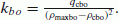
Both cases are part of the congested phase and forced regime (Section 5.2), with a leader speed equal to zero (ν l (x, t) = 0). The model then takes the form

We have, here, an exponential decrease in speed, with τ s as time constant, until the traffic stops. The traffic flow reaches a stationary state corresponding to

5.4 Congested phase and free regime (ρ c < ρ < ρmax)
Suppose that the traffic flow has been disrupted by an exogenous phenomenon. This can be involuntary and then corresponds to one of the previous cases. Otherwise, it is voluntary, i.e. a consequence of traffic control policy that we will discuss further. In both cases, the traffic flow leaves a congested phase (metastable state).
The phase presented here corresponds to the behaviour of downstream front of traffic flow after the disappearance of the disturbance. In other words, this represents the flow behaviour from the exit of the metastable state to the free flow phase. In this case, both state variables coexist, and we suggest using the representation Eq. 20

This corresponds to a congested phase, but with a free regime in the sense that there is no external action on the system. The system returns to the critical state intrinsically (i.e. drivers accelerate to reach their cruising speed). Indeed, in this case we have a second order system with oscillatory behaviour. However, as soon as the density reaches ρ c value, the “potential” energy vanishes and the system switches to a free flow behaviour governed by a first order model.
6 Numerical scheme and simulation
6.1 Numerical scheme
Let us recall that the model obtained is an hyperbolic system in a non-conservative (primitive) form. The corresponding equations are

where

The eigenvalues of A(u) are real and f(u) is a source term which take different expressions according to the phase concerned.
The nonconservative product  makes the integral resolution difficult because of the definition to a weak solution of the problem Eq. 30. Indeed,
  corresponds to two distribution products which does not allow a weak solution of the problem in the classic distribution framework. In the present work,we have used numerical scheme based on the definition of the weak solution given by [9]. In fact, the authors use the concept of a family of paths φ(s, u
g
, u
d
) to define weak solutions for hyperbolic systems in non-conservative form. Choosing a path connecting the left and right sides (respectively u
g
and u
d
) of the discontinuity can consider the product
corresponds to two distribution products which does not allow a weak solution of the problem in the classic distribution framework. In the present work,we have used numerical scheme based on the definition of the weak solution given by [9]. In fact, the authors use the concept of a family of paths φ(s, u
g
, u
d
) to define weak solutions for hyperbolic systems in non-conservative form. Choosing a path connecting the left and right sides (respectively u
g
and u
d
) of the discontinuity can consider the product  as a Borel measure [9, 25]

We also have the following definition: [3, 24]
Given a family of paths φ, a matrix function A φ is called Roe matrix if it satisfies
-
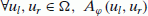 we have N=2 real eigenvalues
 -

-
∀ u l ,u r ∈ Ω ,
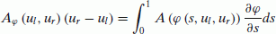 (32)
(32)
 we have N=2 real eigenvalues

Here, we choose the simplest path i.e. segments given by

So, Eq. 32 becomes

Thereafter, we have used an extension of PRICE (PRImitive CEntred schemes) [3]. The approximation of Eq. 33 is ensured by Gauss–Legendre quadrature with three points:

We reach an extended PRICE scheme, where I is the identity matrix (2 × 2) [3]

with

and

It is a scheme with the CFL stability condition.
Remark
The CFL condition states that  must be less than or equal to one.
Let VCFL = νmax in an anisotropic model case and  in PW model case, where c0 represents the sound speed in PW model.
So, to obtain the same accuracy δx in both cases, we must have the following equality:

In other words, the simulation of PW model requires more time.
6.2 Simulation examples
We have to use particular approximation algorithms [3, 25]. Hereafter, we present numerical simulation of some cases.
We consider position x ∈ [0, lg], where lg represents the length of the considered section of road. As in the decomposition methods approach (compare for instance to [12] and [18]), this considered section is divided into several parts, with variable lengths, according to phases concerned. The moving boundaries link these parts, between them, by boundary conditions of Dirichlet type. On the other hand, the conditions of Neumann type are used at x = 0 and x = lg. Then, a front tracking is made according to time evolution [22]. Hereafter, we present numerical simulation of some situations that show agreement between experimental data and model proposed.
6.2.1 Example 1
This example illustrates the evolution of a cluster when the light turns red, at a traffic light, at time r-l and then turns green at time g-l. We have at the same time two phases, free and congested, connected by a moving boundary (systems (22) and (29)). Curves show clearly the evolution according to time of the junction between them. Once the critical density is reached, the system switches to the free flow (Fig. 1).

First example: traffic light
Numerical values used for this example: lg(road length) = 1 km
ρ c = 40 vehicles/km | ρmax = 100 vehicles/km |
ν c = 30 km/h | νmax = 50 km/h |
time r-l = 6.5 s | time g-l = 41.5 s |
6.2.2 Example 2
We show in this example the behaviour of traffic flow in the presence of a vehicle rolling at low speed (less than ν c , Fig. 2):
The specific numerical values for this example are: lg(road length) = 100 km
ρ c = 40 veh./km | ρmax = 100 veh./km |
ν c = 90 km/h | νmax = 130 km/h |
ν l = 40 km/h | position-in= 20 km |
time-in = 40 s | time-out= 78 mn |

Second example: traffic flow behaviour in the presence of a slow vehicle
7 Conclusion
We have proposed a model built on energy principles. It has allowed us to give prominence to the multi-phases behaviour, free and congested flows with their various cases. The conditions of transition between phases appear more clearly because they depend on classic characteristics of the road in question (ρ c , ν c , ρmax, etc.) unlike some anisotropic models as [1, 4, 6, 7, 10]. In the congested traffic case, the model takes into account transient and stationary regimes. This led to differentiation between representations of traffic flow behaviour at the upstream of the congestion, within it, and at the downstream of the congestion. Besides, the cases of total traffic flow blocking can be represented by the model. However, the system becomes more complex. Indeed, having different patterns on adjacent sections of the same road requires the use of special techniques. Nevertheless, the use of methods such as domain decomposition, combined with parallel computing, would overcome this difficulty.
The simulation examples presented above show that the approach is promising. Nevertheless, further works must be made to fit this model to real data [23]. The resulting model has to be improved, notably by a better constant choice in Eq. 14 and has to be completed to take into account junctions and ramp access, for instance.
References
Aw A, Klar A, Rascle M, Materne T (2002) Derivation of continuum traffic flow models from microscopic follow-the-leader models. SIAM J Appl Math 63(1):259–278
Aw A, Rascle M (2000) Resurection of second order models of traffic flow. SIAM J Appl Math 60:916–938
Canestrelli A, Siviglia A, Dumbser M, Toro FE (2010) Well-balanced high-order centred schemes for non-conservative hyperbolic systems. Applications to shallow water equations with fixed and mobile bed. Adv Water Resour 33:291–303
Colombo RM (2002) A 2 × 2 hyperbolic traffic flow model. Math Comput Model 35(5–6):683–688
Colombo RM (2003) Phase transitions in a traffic flow model. Proc Appl Math Mech 3(1):20–23
Colombo RM, Goatin P (2007) Traffic flow models with phase transitions. Flow Turbul Combust 76:383–390
Colombo RM, Goatin P, Priulic FS (2007) Global well posedness of traffic flow models with phase transitions. Nonlinear Anal 66:2413–2426
Daganzo C (1995) Requiem for second-order fluid approximations of traffic flow. Transp Res Part B 29(4):277–286
DalMaso G, LeFloch P, Murat F (1995) Definition and weak stability of nonconservative products. J Math Pures Appl 74(6):483–548
Goatin P (2006) The Aw–Rascle vehicular traffic flow model with phase transitions. Math Comput Model 4:287–303
Greenshields B (1935) A study in highway capacity. Highway Res Board Proc 14:448–477
Herty M, Sead M, Singh AK (2007) A domain decomposition method for conservation laws with discontinuous flux function. Appl Numer Math 57:361–373
Helbing D (2001) Traffic and related self-driven many-particle systems. Rev Mod Phys 73:1067–1141
Hoogendoorn SP, Bovy PHL (2001) State-of-the-art of vehicular traffic flow modelling. J Syst Control Eng 215:283–304
Kerner B (2004) Three-phase traffic theory and highway capacity. Physica A 333:379–440
Lebacque JP et al (2008) Modelling of motorway traffic to second order. C R Acad Sci Paris Ser I 346:1203–1206
Lighthill M, Whitham J (1955) On kinematic waves. I: flow movement in long rivers. II: a theory of traffic flow on long crowded roads. Proc R Soc A229:281–345
Magoules F, Rixen D (2007) Domain decomposition methods: recent advances and new challenges in engineering. Comput Methods Appl Mech Eng 196:1345–1622
Michalopoulos PG, Yi P, Lyrintzis AS (1993) Continuum modelling of traffic dynamics for congested freeways. Transp Res Part B 27(4):315–332
Morrison PJ (1998) Hamiltonian description of the ideal fluid. Rev Mod Phys 70(2):467–521
Nakrachi A (2009) On traffic flow modelling with phase transition: an energy concept. In: 12th IFAC symp. on transp. syst. Redondo Beach, CA, USA, 2–4 Sept, pp 346–351
Nakrachi A, Popescu D (2010) Modelling and simulation of macroscopic traffic flow: a case study. In: 18th Med. conf. on cont. and auto. Marrakech, Morocco, 23–25 June, pp 1626–1631
Papageorgiou M (1998) Some remarks on macroscopic traffic flow modelling. Transp Res Part A 32:323–329
Pares C, Castro M (2004) On the well-balnce property of Roe’s method for nonconservative hyperbolic systems: application to shallow-water systems. Math Model Numer Anal 38(5):821–852
Pares C (2006) Numerical methods for nonconservative hyperbolic systems: a theoretical framework. SIAM J. Numer Anal 44:300–321
Payne HI (1971) Models of freeway traffic and control. Math Models Publ Sys Simul Council Proc 28:51–61
Pronko G (2006) C2 formulation of Euler liquid. Theor Math Phys 148(1):980–985
Richards PI (1956) Shock waves on the highway. Oper Res 4:42–51
Whitham GB (1974) Linear and nonlinear waves. Wiley, New York
Zakharov V (1971) Hamiltonian formalism of hydrodynamic plasma models. Sov J Exp Theor Phys 33:927–933
Zhang H (2002) A non-equilibrium traffic model devoid of gas-like behaviour. Transp Res Part B 36(3):275–290
Author information
Authors and Affiliations
Corresponding author
Appendix
Appendix
1.1 A. List of the abbreviations and symbols
AR | Aw and Rascle model |
LWR | Lighthill, Whitham and Richards model |
PW | Payne and Whitham model |
CFL | Courant Friedrichs Lewy |
ε | internal energy per length unit |
ρ c | critical density |
ρ max | maximum density |
e t | total energy per length unit |
e k | kinetic energy per length unit |
ν c | critical speed |
ν max | maximum speed |
V e ρ) | equilibrium speed |
T PW | reaction time |
1.2 B. Determination of c value
Integrating Eq. 12, we obtain an expression of total energy, for ρ c ≤ ρ ≤ ρmax,

where L represents the length of the road in question.
To obtain the expression of c, we write this total energy for ρ = ρ c , which is a constant

and for ρ = ρmax

we obtain the expression

Rights and permissions
Open Access This article is distributed under the terms of the Creative Commons Attribution 2.0 International License (https://creativecommons.org/licenses/by/2.0), which permits unrestricted use, distribution, and reproduction in any medium, provided the original work is properly cited.
About this article
Cite this article
Nakrachi, A., Hayat, S. & Popescu, D. An energy concept for macroscopic traffic flow modelling. Eur. Transp. Res. Rev. 4, 57–66 (2012). https://doi.org/10.1007/s12544-012-0070-0
Received:
Accepted:
Published:
Issue Date:
DOI: https://doi.org/10.1007/s12544-012-0070-0