- Original Paper
- Open access
- Published:
A proposal for an operating cycle description format for road transport missions
European Transport Research Review volume 10, Article number: 31 (2018)
Abstract
Purpose
This article presents a proposal for an operating cycle format for describing transport missions of road vehicles, for example a logging truck fetching its cargo. The primary application is in dynamic simulation models for evaluation of energy consumption and other costs of transportation. When applied to product development, the objective is an ensemble of components and functions optimised for specific tasks and environments. When applied to selection of vehicle configuration, the objective is a vehicle specification tailored for its task.
Method
The proposal is presented and its four main parts: road, weather, traffic and mission, are thoroughly explained. Furthermore, we implement the proposal in an example of a dynamic forward simulation model.
Results
The example model is used for two case studies: a synthetic example of a complex transport mission (a logging truck fetching its cargo) that shows some advanced format features, and an example from a real vehicle log file (cargo transport) that seeks to compare the resulting simulated speed profile to the measured one.
Conclusion
The results show that the proposed format works in practice. It can represent complex transport missions and it can be used to reproduce the main features of a logged speed profile even when combined with simple driver and vehicle models.
1 Introduction
Accurate prediction of energy consumption and vehicle performance, in the pursuit of CO2 reduction and fuel saving, is a challenging task. Simulations require detailed models of the vehicle and its control systems, and a great deal of effort has been put into this, both by original equipment manufacturers and governmental agencies. However, regardless of how detailed the vehicle model is, the prediction will be misleading unless it is excited in the right way by the right physical entities [1]. Naturally, the driver and environment are the cause of the excitations, and the focal point of this study is the question of how to describe the environment. We refer to this as ‘the representation problem’.
In traditional and simple simulation modelling environments, the vehicle moves forward along a ‘straight’ line. Among the many examples in this category is VECTO [2]. It is becoming increasingly evident that many of the important control systems on modern vehicles rely on more accurate descriptions of the vehicle motion to be able to show good correlation between simulation and measurements. Examples of such systems include energy storage, charging, systems providing external loads such as cranes and pumps, clutches, transmissions, and emission control. To extend the modelling space, one can consider the example of a logging truck going into a forest site to pick up timber logs and transporting them to the next step in the wood production process. Typically, the logs are gathered deep in the forest and it is beneficial if the truck can go far in to pick them up. As roads get increasingly narrow and soft the farther into the forest it goes, a heavy-duty truck may need to change its driving direction at the last possible point, and reverse the last distance to the point of pick-up. This is illustrated in Fig. 1.

The logging truck mission
A common way to perform vehicle simulation is to use speed as a function of time or position (a driving cycle) to stimulate the vehicle model [3, 4] (Fig. 2). This is a problematic approach. It has become obvious that those methods have serious drawbacks:
-
A
The comparison problem: how to compare vehicles with different propulsion systems?
Fig. 2 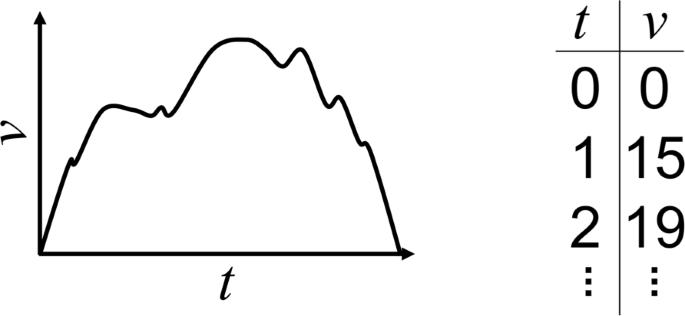
An archetypical driving cycle
-
B
The 24/7 problem: many systems depend on what happens during the entire day, with much standstill and idling; how can that be described?
-
C
The technology problem: how can new inventions be included and described? Charging stations, for example.

In this paper, we propose an operating cycle format, which can contain a representation of the road, the weather, the traffic and the mission. It should be sufficiently detailed that it can excite the vehicle in the appropriate way and, at the same time, sufficiently simple to allow for easy design based on log data, road map databases, stochastic generation or other methods.
The intended use of the operating cycle format is in a composite simulation model, as in Fig. 3, for prediction of energy consumption, CO2-emission and longitudinal performance.

Basic top-level structure of a modular forward simulation
The overall purposes could be many, but here we have in mind evaluation of vehicle performance, specifically the powertrain system, where the results can furthermore be used in both product development and selection of vehicle configuration.
In the context of development, well defined transport missions can be used to tune functions, individual components and the complete system, to avoid extensive prototyping. Correctly used, it enables development of functions (such as gear shift strategy and eco-roll) that are optimised for the best fuel economy and lowest CO2-emission based on application. Likewise, components and sub-systems (like the clutch and the gearbox) can be constructed and evaluated for specific tasks and environments. Not only does this lead to better performance than if the component was developed for every possible task and all environments [5], but it may also lead to recommendations on where and what application the system is suitable for [6]. It simplifies the sales-to-order process when choosing vehicle configuration by reducing the number of dimensions in the optimisation domain. That selection process is the second example: the most suitable powertrain configuration for individual users can be found through software simulation, if the characteristics of both the transport mission and the driver are known, in theory. This would result in a vehicle specification that is fuel optimal based on how it is actually used by the customer, with respect to the set of available systems. In practice, the optimisation problem is difficult to solve because of the vast number of possible component and function combinations (see e.g. Nedělková et al [7] or Lindroth [8]).
In both cases, a proper description of the transport mission is necessary for the composite simulation model to reproduce real-world behaviour. However, the level of detail of the driver and vehicle models of course affect the accuracy of the predicted energy consumption. In addition, the driver’s style of driving can have a major effect and may contribute with a variation of around 10% [9] in CO2-emissions for a given vehicle and travel route. These are separate issues, and provided that the composite simulation model has the structure in Fig. 3, they can be treated independently of the representation problem discussed here.
The structure of the paper is as follows: firstly, we present a literature survey and discuss existing mission descriptions in Section 2. Secondly, the format proposal is defined and its parts are explained in Section 3. Next, in Section 4 an implementation into a dynamic simulation model is made and described. The composite model was applied to two case studies and the results are presented in Section 5.
2 Previous work
The topic of transport missions is sparsely mentioned in academic literature, but there are some descriptions of the road and mission. In this section, we make a brief review.
For vehicle simulators, the format OpenDRIVE [10] has successfully become something of a standard. This is a description of the road infrastructure: the geometry of the road including lane width, road signs, etc., and can also contain information on road surface if coupled with its sister format OpenCRG [11]. OpenDRIVE has been around since 2007 and offers an extensive description of a road network. However, it is not intended to describe actions on the road: details such as where to start or stop, to load or unload, or where and how to use auxiliary equipment must come from another source. Other formats with the explicit purpose of describing a road network exist, but suffer from the same disadvantage.
The most basic form of a transport mission description is a conventional driving cycle, where the speed is either a function of position or time (Fig. 2). Although this is a very simplified way of seeing the mission it is popular to use, especially for benchmarking, rating and regulation (see, e.g., [12,13]). An obvious downside with this basic description is that the impact from the surroundings is missing. A subtler problem arises because of the fundamental idea to prescribe the vehicle speed exactly. Since the profile is given, the acceleration is stipulated too. In a simulation, it has the consequence that a change in vehicle configuration is not allowed to influence the speed or quantities related to it, such as transport efficiency. For example, changing components to increase the acceleration performance (such as choosing a more powerful engine or higher gear ratio) would have no impact: a vehicle that could accelerate more quickly is not allowed to because of the prescribed speed. For the same reason, advanced functions that use speed variation as a tool to improve fuel economy (for example by using the vehicle itself as an energy buffer when negotiating hills [14–17]) are not allowed to influence the outcome. Therefore, a driving cycle does not allow for a fair and objective evaluation: the comparison problem mentioned in the introduction.
Many simulation software packages, whether commercial or free, have their own way of describing the road and mission: often by combining a traditional driving cycle with one or more road parameters, such as topography (see, e.g., [2,18,19]).
There are also transport mission descriptions that are of an entirely different kind. The high-level description offered by the Global Transport Application (see Edlund and Fryk [5]) is one example, where the mission is divided into different classes based on statistical measures. Similarly, there are many approaches to Markov-based methods, for example: Johannesson et al [20], Nyberg [1] and Speckert et al [21], where the mission is described in terms of parameters belonging to one or several stochastic models. These types of high-level descriptions cannot excite a vehicle model by themselves, but instead use an intermediary step: often by generating data to a conventional driving cycle.
3 Format proposal
We start by defining a transport mission as an enumerable number of tasks (the mission) that take place in certain surroundings (road, weather and traffic), independent of both driver and vehicle. For example, it could be a bus timetable and a number of passengers inside a city core; or a load of sand being picked up at a position, driven to a construction site and then distributed over a distance; or just a series of pickup and drop-off points with a number of parcels along a country road. The challenge is to determine what to describe and how to do it mathematically.
Furthermore, the intended final use is to predict energy consumption and performance, so any effect that has a significant impact needs to be included. To gain an idea of what to look for, we start by rewriting Newton’s second law slightly, Eq. (1)
The propulsion power P prop is supplied by the vehicle power source (see Appendix 1 or [22]); if a proper description of the elements on the right-hand side of Eq. (2) is found, the initial goal will be met. We refer to each such descriptive term as a parameter; these are described in Sections 3.1-3.5 together with Table 1, and illustrated in Fig. 4. All symbols and variables are explained in Table 9, Appendix 3.

An illustration of the structure of the OC-format proposal
Additionally, the format must satisfy several guiding principles. It needs to be easy to use when designing missions, computationally efficient during simulation, independent of both vehicle and driver, compact, completely deterministic, and all components must have a physical interpretation. We call this the operating cycle format, so a transport mission description on this form is called an operating cycle (OC).
3.1 Parameter structure
Each parameter corresponds to a physical quantity, denoted by p, that is either a function of position along the trajectory x, time t or both. The value of p is specified at a discrete set of points and given as an array P, together with either an associated array of positions X, times T or both, such that
An underlying mathematical model for interpolation must also be specified to describe what happens for intermediary values x∈]X i ,Xi+1[ and/or t∈]T j ,Tj+1[. The positions included in the table are to be interpreted as the position along the trajectory; that is, the arc length of a reference point (perfectly) following the path. Therefore, the points need to be arranged in increasing order. Note that different parameters do not have to be specified at the same points in space or time.
The suggested model for each parameter is listed in Table 1. Here, the term ‘linear’ means piecewise linear, and ‘constant’ means (right side continuous) piecewise constant. The parameters termed as ‘discrete’ describe singular events that have a specific position (or point in time), such as a stop sign, but have no continuous effect before or after this point. The mission category parameters are given in a different way, but can be rewritten in the above form (see Section 3.5).
An explicit example of an OC is shown in Section 5.1 and Appendix 2.
3.2 Road
The parameters in the road category describe the time-constant infrastructure and the physical properties of the road, including the geometry. Road signs that always require a driver to behave in the same way are included, but signs that require different action depending on the presence of other vehicles belong in the traffic category. For example, a stop sign always requires vehicles to stop at the given position and belongs in the road category. A give-way sign prescribes action to either stop or continue depending on the traffic situation and belongs in the traffic category.
Speed signs, stop signs and road bumps correspond to the physical entities after which they are named. All three have a major influence on the speed, and hence the inertial force. Stop signs are discrete entities that are characterised by a position and a standstill duration. Speed bumps are also given at discrete positions, but are instead described by a length l, a height h and a (maximum) deflection angle α. On roads where there are no speed signs, a default speed based on local regulations should be given instead.
The topography describes the altitude; that is, the equivalent to the vertical z-coordinate in a local Cartesian coordinate system. It is included to describe the slope resistance and has a major impact on energy usage.
The curvature parameter represents the curvature of the trajectory in the road plane. The main reason for its inclusion is that it affects the driver’s choice of speed. It also has a direct effect on energy consumption and performance since the vehicle loses energy due to side slip, but this is small enough that it can be neglected in most cases (see e.g. Jacobson [23]).
The ground type describes the road surface in general terms. It has two entries: type G t and cone index CI (see Wong [24]). The type is a unitless integer that points out the type of ground: tarmac, grass, clay, cobblestone, etc. The cone index is a measure of the bearing capacity of the ground.
The intention is not to describe the physical surface and soil properties in detail, which is a complex task (see Contreras et al. [25] for a review) and of limited usefulness. The parameter must be used to calculate information that is vehicle-dependent, such as: rolling resistance coefficient or friction coefficient. Those interactions are all heavily tyre-dependent and cannot be included directly in the OC description without violating the guiding principle of vehicle independence. By describing the ground this way instead, it is straightforward to include empirical data for specific tyres or physical models (such as those suggested by, e.g., Harnisch et al. [26] or Wong [24]) that do describe tyre-soil interactions. Figure 5 explains how this works.

The top-level structure of the simulation model and the relation between an OC and its counterpart in the dynamic simulation
The road roughness is described using ISO8608 [27]: degree of unevenness C and waviness w. Although roughness is generally considered mostly when assessing fatigue and comfort [28], it can also affect the choice of speed. In addition, there is a direct effect on energy consumption because of dissipation in the suspension dampers (see Jin-Qui et al [29]).
The longitude and latitude are given by their WGS84 counterparts. The GPS-coordinate entries are different in nature to the other parameters. The reason for their inclusion is that many advanced systems make use of positioning data to adapt vehicle behaviour in the form of gear selection, speed choice, engine on/off, etc., to increase performance in various ways. Fuel economy is a common thing to improve with such systems; see e.g. [14–16]. The GPS-coordinates could be computed from the geometric trajectory given an initial coordinate and direction, but it is a numerically sensitive process, both when constructing the OC and in practical simulation.
Other energy-relevant parameters could also be included, such as lateral road width, side width, number of lanes and super elevation. They would mainly affect the choice of speed.
3.3 Weather
The weather category describes the time-constant physical properties of the surrounding apart from the road itself. It can be thought of as any parameter that affects the vehicle performance but is not caused by the road or other vehicles. These parameters are taken as functions of position only. Exceptionally long missions, stretching over a day or more, would be affected by the time variation and could sometimes require its inclusion.
The ambient temperature and atmospheric pressure describe the corresponding physical properties of the surrounding.
The wind velocity v w =[v wx ,v wy ] is a two-component vector. It is defined in a global, fixed-coordinate system.
The relative humidity is the amount of water vapour in the air, measured as a percentage (of partial water vapour pressure to equilibrium water vapour pressure; see, e.g., chapter 12.1 of Green [30]).
One may reflect that these parameters are not independent of each other or of parameters in other categories. For example, the atmospheric pressure decreases with the altitude, while the humidity decreases with temperature (isobaric heating) but increases with pressure (isothermal heating). Whether those dependencies need to be modelled depends on the origin of the data being used.
Apart from the wind velocity, the weather parameters do not contribute with direct resistive forces. They do affect how well the vehicle power source works and they indicate that other power users may also be needed (air conditioning, headlights, windscreen wipers, etc.).
Other possible properties, such as visibility, could be included as well.
3.4 Traffic
This category intends to contain parameters that can describe the impact from surrounding vehicles, as well as signals or signs that prescribe rules that include other vehicles. Some of these have comparatively short time dependence, changing over seconds, minutes or hours. They could include both a position and time dependence.
Traffic is problematic to describe from the point of view of a single vehicle. Normally, statistical methods are used, a subject of traffic flow theory (many textbooks are available; e.g., Elefteriadou [31]). The parameter that is included here barely scratches the surface and should be regarded as a place holder for a more detailed description.
The traffic light and give-way sign are defined by their position and given as discrete entries together with a stop time. The result is that the entries are identical to that of a stop sign. This is not a bad thing: it is a valid model for red and green light (entry with zero stop time), but it does not reflect the stochastic nature of a real stop light.
The traffic density is the number of vehicles per length unit. Alone, this parameter is not sufficient to describe influence of traffic on the vehicle speed; instead, it serves as an example of what parameters that can be included. The consequence is that the OC-format cannot describe a mission where the surrounding traffic has a non-negligible impact on the subject vehicle. This is an important limitation of the proposed description in its current form, with the consequence that only missions in calm traffic situations are suitable to describe with the presented method.
To have an impact in a simulation, traffic density and vehicle speed must be connected. This presents a problem: the perspective here is from a single vehicle, often called the picoscale, which is not normally used by itself to model traffic. Instead, it is coupled to other vehicles via a car following model, but that requires simulation of those vehicles and therefore a different approach to the modelling procedure. That type of modelling perspective is usually called the microscale. There have been some interesting attempts to combine the picoscale and microscale (see Ni [32]), which could prove fruitful.
An alternative way to describe the impact of traffic is by using empirical data. Some map databases [33,34] list mean traffic flow speed with reasonable resolution in both position and (clock) time. That data could be used directly in a simulation without having to go via a density. A disadvantage is that only static limits come out, missing out on the rapid variations.
3.5 Mission
The parameters in this category should reflect the reason why the vehicle is on the road. Most missions involve the transportation of either goods or people, but there are plenty of accessories that can be utilised during the trip.
The mission category is different from the others. The parameters here can change during standstill, and cannot be specified only with a position or a time; instead, a time duration or a trigger from the driver is needed. However, it must still be possible to include position dependence simultaneously so that they are able to vary during motion.
One solution is to gather all parameters into a matrix M, called the mission matrix, and allow each entry to be specified with both a time duration and a position. Each row in the matrix can be written
where X i and ts,i are the position and time duration of each row etc. We may write the entire matrix as M=[m i ]i=1,…,N. If the action is to be performed during a stop, then the entry’s position is identical to the previous one. If the action is triggered by position, the time duration is zero.
The downside is that the description in this category is less compact. Whenever one parameter changes, all must be specified and redundant information is included. Another disadvantage is that some measure of pre-processing is usually needed to separate the position and time dependence before the information can be used in a dynamic simulation model.
The mission stop parameter s m is a Boolean that denotes whether the entry is to be conducted during a stop (TRUE) or while in motion (FALSE). If it does denote a stop, then the standstill duration entry must be nonzero. Furthermore, a position must always be given, even if there are several actions during the same standstill session.
The cargo weight is the weight of the cargo (payload).
The power take-off parameter P PTO describes the power demand from one or several accessories fitted on the vehicle. This could be anything from a freezer that is active during the entire trip, to a crane that is only used for loading cargo during standstill. The direction of power is a flux from the vehicle to the accessory, so a positive value means power from the vehicle energy well.
Similarly, the charging power parameter P in describes the maximum power available for charging. The direction of power is a flux from the charging machine to the vehicle; therefore, a positive value means power to the vehicle energy well. The choice of a piecewise constant function is intended to enable description of charging along the road (power supply lines drawn above it, rails in the road plane or inductively). At present, the most common use would be to have discrete charging stations, but that is easily modelled (though non-compact) using three stop entries.
The travel direction parameter e d indicates whether the intended travel direction is forward (1) or reverse (−1). Reversing is a manoeuvre that is often neglected in simulations of powertrain concepts and configurations.
The mission matrix can be broken up and each parameter given as a table, in the same way as explained in the beginning of the section. The problem is that all the parameters need to be given at all positions and with a time duration, which means that the results would include even more redundant information.
3.6 Formal definition
Formally, the OC becomes the set that contains all parameters. If the four categories are defined as

then the OC  is the combination of these sets,

This set, together with the mathematical model listed in Table 1, forms the core of the format proposal.
4 Implementation
To demonstrate what an implementation of an OC may look like in a dynamic model, an example was constructed. The structure of the composite model is shown in Fig. 5: it is a forward simulation that consists of the OC, a driver and a vehicle, that all follow the general principles outlined in Pettersson et al. [6]. In the figure, the boxes on the lower level correspond to the dynamic models and the arrows show the signal flow between them. The modules on the upper level assign values to the parameters in the simulation model, and lines with dots at the end show parametrisation interfaces.
We would like to emphasize again that the OC is the novel and interesting part here, together with the driver interpretation. The operative driver and the vehicle are necessary to model for the simulation to run, but they are only intended as examples and are therefore kept as simple as possible. The downside is that the accuracy of natural validation measures, like CO2-emission, fuel consumption and total amount of energy used, is questionable. The details are not reliable so we will settle for order-of-magnitude estimates. More realistic and accurate results could be obtained by increasing the complexity of the driver and the vehicle, but that is not the purpose here.
4.1 Operating cycle model
The main module is shown in Fig. 6. The system has been separated into the four categories to make for an easier overview, although that is not necessary functionally. The road, weather and traffic submodules all work in the same way; the signal values at the current vehicle position are found by interpolation using the mathematical model in Table 1. Some of the upcoming parameter values and the position of the change are also sent onwards.

Stylised example of an OC implementation: the main module is in the top-left, the middle green circle shows how the mission is implemented, and the state machine is shown inside the red circle
The handling of the mission (Fig. 6, right) is more complex because it can be active both when driving and during standstill, but must function differently depending on which variable governs the mathematical model: position or time. The ambiguity is resolved by looking at each stop as an event, regardless of whether it is due to the mission, a stop sign, a traffic light or a give-way sign. At each event, the mission matrix is scanned through to see what actions, defined by identical positions (say N), are to be performed. A new matrix, the action matrix A, is created where the time duration t s of each relevant entry in the mission matrix is used to form a cumulative time array T.
each row in the action matrix can then be written as
and the matrix itself
This is used together with the underlying mathematical model in Table 1 to determine the output at standstill. There is one matrix for each stop: if there are no actions to perform during standstill, the stop is considered trivial but still has an action matrix. When driving, the handling of the parameters is identical to the road, weather and traffic subsystems.
Finally, there is a subsystem that determines whether the standstill or the driving module should be active; this is the state machine in Fig. 6. There are two states, ‘Driving’ and ‘Standstill’, which naturally refer to the modules with corresponding names. In addition to controlling which subsystem is active, the state machine also keeps track of the next stop (which action matrix to use), and sends out a Boolean flag that signals the driver model when a stop task is completed. The transitions between the states are based on the distance to next stop d s , the vehicle speed v and the total time in each stop T N .
The last thing that needs to be mentioned is how to treat the position of the vehicle when reversing. There are three possibilities
Equation 13 would be the right choice if the trajectory was in one dimension, but here it is embedded in three dimensions. The obvious solution is to take all spatial dimensions into account, but then the parameters in the OC-format would need to be specified in space instead of along the line, which would be an unnecessary complication and highly non-compact.
Equation 14 is the arc length, the total travelled distance. It does not suffer from the above problem since it is independent of the direction of motion. However, unintentional motion in the wrong direction, such as backwards slip when starting, would be mistaken for motion in the forward direction. A larger problem is that a simulated vehicle will never stop exactly where intended. Therefore, if the travelled distance is used as a position indicator when switching driving direction, there will be an error whose size is the difference between intended and actual stop distance when compared to the OC. Consequently, the physical parameters (such as topography) will not be computed at the correct points, which would cause problems when comparing vehicle configurations as all vehicles would drive a slightly different road.
The suggested solution is to see each trip between stops as its own segment, as in Eq. (15). Then each segment would have a constant travel direction and the position could easily be tracked as if it was only in one dimension. Unintended motion is still accounted for, and travel in the intended direction results in a monotonously increasing position. If the position is kept track of within each segment, it is easy to compensate for stopping out of position by comparing actual and target distance. The downside is that even when describing true one-dimensional motion, both the forward and backward trip must be described. Thus, there is a risk that the same stretch of road is parameterised differently unless care is taken when constructing the OC.
Note that Eq. (14) still describes the total distance travelled and should be used when evaluating measures per distance.
4.2 Driver model
A point to note when comparing the OC-format to conventional driving cycles is that there is no target speed. While the speed signs do provide an upper limit, they say nothing about the level of acceleration. Furthermore, there are many cases in which it is not appropriate or possible to maintain that speed; examples include sharp curves, roundabouts, approaching intersections, behind other vehicles, speed bumps, and low friction conditions. We approached that problem by splitting the driver model into two parts: a high-level driver who translates (some of) the OC-parameters into a desired speed, and a low-level driver who controls the output to the vehicle - here in the form of accelerator and brake pedal - based on the error between the wanted and the actual speed. Figure 7 shows an outline.

Top level of the driver model
The division into two parts is similar to the ideas of Eriksson [35], where there is a strategicFootnote 1 and an operative part. The operative part works towards limits and set-points, using the accelerator pedal and brake pedal to reach the control objectives set by the tactical part. The tactical part works with things like suitable levels for acceleration and deceleration and has a wider view on the driving task.
We wish to emphasize that the OC-format says nothing about the driver. They are different entities and can be modelled separately, but they do communicate with each other. Furthermore, the driver model here is not a complete description of a human driver and it does not reflect the driving style of any person in particular. It is simply one example of an implementation where a driver uses some of the information provided by the OC.
4.2.1 Interpretive part (tactical)
In this implementation, the parameters that have an influence (called active parameters) are: speed signs, stop sign, give way sign, traffic light, mission stop, curvature, and speed bumps. The first four parameters are related to legal requirements, while the latter two are of a physical nature and touch upon the driver’s sensitivity to lateral and vertical acceleration (see Karlsson [36] and Reymond [37]).
Several other parameters could be included in the second category: roughness causes vertical acceleration, and ground type affects road grip. Neither of them are considered in this paper because they had no or negligible influence on the case studies here (see Section 5).
The speed threshold suggested by the active parameters are as follows: the signed speed is an immediate threshold: v sign . The stop sign, give way sign and traffic lights all enforce full standstill: v stop =0 m/s, centred in a small region around the stop position. For the curvature, we imagine that the driver has a maximum lateral acceleration limit, |a y |≤ay0, above which he or she is not comfortable driving. The kinematical relationship implies a speed limit
An empirical relation is used to explain speed humps based on the results by Johnson et al. [38]: a mean speed V b is observed for a certain bump type with given height, length and geometry. In this paper, we assume a model that varies with the bump deflection angle α as
This function has been chosen for its asymptotic behaviour: if the bump deflection angle is 0 then it should have no impact on speed, but if it is a vertical step then only a small speed should be allowed. The constants C1 and C2 are chosen such that v b (α0)=V b and \(v_{b} (\pi /2)=V_{b}^{min}\).
In addition, the active parameters are all visible to the driver and allow for some measure of planning. For example, the driver can see that there is a sharp curve ahead, and will adjust his or her speed. So, a predictive part is included, combined with a constraint on the minimum acceleration (maximum deceleration): a x ≥−ax0, that the driver is comfortable with. Thus, the upcoming value of each active parameter Xi+1, Pi+1 supplies a predicted maximum speed \(v_{p}^{\prime }\) too
Where vp,i+1 is the associated speed limit of parameter p at Xi+1. To make a final choice of desired speed, we imagine that the driver will want to drive as fast as possible, subject to both current and predicted maximum speed thresholds
With our choice of active parameters, it becomes
One case where the above equation reflects the vehicle behaviour poorly is during a reversing manoeuvre; very few drivers would drive at the speed limits while going in reverse. In such cases, another, static speed parameter is considered (v rev ) and other limiting values for ay0, ax0 are used.
4.2.2 Control part (operative)
The control part of the driver is a much simpler concept: the interface to the vehicle is an accelerator pedal and a brake pedal, normalised such that a p ,b p ∈[0,1]. The desired speed v want is compared to the current vehicle speed v and a PID-controller is used to control the pedal output based on the error. This kind of description makes no attempt to model the neuromuscular behaviour, but is nonetheless popular for longitudinal applications, like lap-time simulations [39].
To allow the driver to maintain a stable standstill, another state machine is included. It is analogous to that of Fig. 6, except that there is no output apart from the state itself. The transition condition for Driving to Standstill is d s <d max , and from Standstill to Driving it is okToStart==TRUE. In Standstill, the brake pedal is linearly increased in time from its initial value to 1 and maintained. The gearshift reflects an automatic gearbox, where 1 means drive and −1 means reverse.
4.3 Vehicle model
The vehicle model consists of a powertrain model for a conventional internal combustion engine, an ideal stepped gearbox and a simple chassis model. As simple a model as possible has been used for this paper. More advanced models, inspired by Berglund [40], have also been tested successfully. The mathematical details can be found in Appendix 1.
5 Simulation and results
Two scenarios have been considered and simulated to show how the format proposal works in practice. The first is the logging truck example in the introduction. Its OC is based on purely synthetic values and is intended to be an example of how a complex mission works and how a synthetic mission can be designed. The second scenario is based on a real truck mission and shows how an OC can be constructed based on those premises and how a simulated mission compares to actual log data from real world driving.
5.1 Synthetic example: logging truck mission
The mission follows the idea displayed in Fig. 1 with five sections
-
1.
From standstill, straight driving to the stop sign and stop.
-
2.
From the stop sign, straight driving onto a turn-off road.
-
3.
Reverse onto the main road, then straight reverse approximately 400 m to the stash of logs and stop.
-
4.
Use crane and load trailer with timber (25 tonnes).
-
5.
Straight driving back to the mission starting point with a stop sign in between.
The parameters that change during the mission are: curvature, stop sign and the mission matrix, all others are constant. The total trip distance is about 3 km and the speed limit is 50 km/h. The mission matrix is shown in Table 2, the rest of the OC is included in Appendix 2. The results of the simulation are shown in Fig. 8.

Plots from the simulated logging truck mission: the top graphs show wanted and actual speed as functions of time and position; the mid plots show the speed around the curve as functions of time and position; the bottom-left plot shows the different position concepts (Eq. (13) in blue, (14) in black and (15) in dotted yellow); and the bottom-right plot shows the power take-off request and cargo mass as functions of time
The speed limit of the entire cycle is fixed, but the curve at x=1.2 km reduces the speed, as shown in the middle graphs. The same plots also show how the reversing works: there is straight line driving for 10 m, then a (quarter-circle) curve again. The lateral acceleration limit has different values depending on travel direction, so the forward and backward speeds in the curve are not identical.
The mid-left plot demonstrates how the three position candidates behave. The difference in arc length and segmented position is only 6.2 m in the end: a difference of 3 m is picked up at the switch at 1.236 km because the vehicle comes to a standstill at 1.233 km, and another 3.2 m when switching back at 1.600 km (because it stops at 1.597 km).
Most importantly, the example shows that the approach of having both distance-based and time (duration)-based parameters works well. In particular, it makes it possible to simulate consecutive actions during standstill: the two bottom graphs show how the total vehicle weight and the PTO (request) develop during the extended standstill session, in total about 10 min.
One point of interest is that the driving part requires a total energy at the wheels of 3.3 kWh, while the crane uses 0.67 kWh to load the timber. Therefore, it would be a mistake to omit the loading scenario, although it is a very short driving distance.
5.2 Real-life example: city outskirt mission
The second scenario originates from a log file of a real truck mission. The data is provided by the operating cycle energy management projectFootnote 2. The mission is a simple transport mission between two locations, without any complications such as reversing or standstill operation. The idea is to see what kind of speed profile results from the OC (and its implementation) and compare it with the logged vehicle. Recall that there is no explicit target speed in the format proposal.
The route of the logged vehicle is shown in Fig. 9Footnote 3, going around the outskirts of Göteborg, Sweden. The starting point was a loading terminal in Sisjön (south-east), then onto a minor highway, with final stop in Lundby (north-west). The route was 17 km long, took approximately 19 minutes on a Tuesday in late April 2014 at around 11:30 a.m. The vehicle in this case was a Volvo FH-16 6x4RADD rigid, with a total weight around 14 tonnes. The resulting speed profile is shown in Fig. 10.

Speed profiles of the three runs. The original 2014 log is labelled OCEAN, while the two new are labelled M2 and M4. The large difference in speed between the log and the measurements at 12-13 km is due to a temporary road work (repairs on the bridge Älvsborgsbron)
The influence of traffic is something that needs investigation given that a systematic description is missing in the OC-format, but the log file contains no direct information about it. Therefore, two measurements were made on approximately the same stretch of road, although in this case both are dated mid-August 2016, at around 8:30 and 9:40 a.m. These were video-recorded for additional documentation and analysis. The vehicle used was a Volvo FH-16 6x4RADD tractor provided by the Revere labFootnote 4. The resulting speed profiles can be seen in Fig. 10. Note that the driver in the two new measurements was not same as the driver in the original log.
An OC was created based on these three measurements. The parameters of interest were the speed limit, curvature, topography, speed bumps and the three stop parameters. The mission matrix is trivial and only shows trip start and end. All other parameters were constant and inactive.
The speed limits were estimated using the video and map data. The curvature was estimated from the GPS-route. In this case, it was not done continuously; only curves with sharp enough curvature were included (13 in total). The topography was estimated every 25 m by using the altitude from the GPS.
There were no stop signs on the route, only traffic lights and give way signs. Figure 10 shows the three speed profiles. There are several differences that reflect the stochasticity of give way signs, but overall the three runs were very similar. All three stopped at the traffic light located at just above the 16-km mark, so this was taken as a red light. The active parameters in the OC is shown in Fig. 11, together with the speed and GPS-altitude from M4.

The active parameters, with comparison from M4. Note the similarities between the speed limits and the M4 speed profile. In the altitude received from the GPS there is a large problem between 10-12 km, due to a tunnel (Gnistängstunneln)
The interesting part is in comparing the resulting speed profile with the measured one; see Fig. 12.

A comparison between the simulation results, including both actual and target speed, and the speed profile from M4. The top-left plot shows the entire trip, while the three others show closer looks in three parts: first part at [0,3.0] km (top right), middle part at [3.0,13.0] km (bottom left) and final part at [13.0,17.2] km (bottom right)
Some things may be noted from these results. Firstly, in this case the speed is mainly governed by the speed limits. Next, there are six instances where the curvature affects the speed greatly: four in first part (0.32, 0.43, 2.2 and 2.7 km) and two in final part (14.9 and 15.6 km). In all cases, the measured speed is lower than the simulated one, perhaps because the acceleration limit needs better tailoring (ay0=0.2g was used) or because the curvature estimate is inaccurate. Another reflection is that the measured speed is at its lowest right before the curve, not in it. This likely reflects a property of the give-way sign in intersections: to avoid stopping completely, the driver controls his or her speed appropriately. This mechanism has not been modelled, but could be since the OC-format provides information about give-way sign locations.
There are some places where the measurement shows significant speed drop but the simulation does not: 2.0 (first part), 4.2 (middle part) and 13.8 km (final part). These were analysed using the video recording. The drop at 13.8 km is due to traffic; a truck switching lanes. The two remaining speed drops, at 2.0 and 4.2 km, are neither due to geometry nor traffic; it just seems that the driver did not watch the speedometer carefully enough.
The simulated speed profile exhibits many small oscillations, mainly due to small changes in topography. They could largely be removed by including another predictive part in the driver interpretation, but it is not necessarily a good thing: much of the variation can be seen in the measured profile as well.
Another reflection from the first and final parts is that the simulated vehicle accelerates more quickly than the real one. This is mostly because of the vehicle model: the real vehicle has an active torque limiter when running unladen to protect the engine and transmission from damage, and the gearshifts are not instantaneous but come with a power disruption. Neither of these effects have been modelled in the vehicle. Recall that the OC-format does not stipulate acceleration in any way.
The fuel consumption can be computed by integration of Eq. (24), and the result is 44 l/100 km (84 g CO2/tonne ·km) for the simulated vehicle. This is a relatively large number: the reason is that the engine often works at a low torque compared to its maximum, and hence has a low efficiency. Unfortunately, a fuel consumption value cannot be given for the mission in the OCEAN log because no signals related to fuel were available. However, we can use the energy produced by the engine as a comparison. In the log file, the total amount of energy produced was 21.2 kWh, leading to an energy consumption of 123 kWh/100 km. The corresponding number in the simulation was 110 kWh/100 km: a difference of about 11%.
6 Conclusion and future work
We have proposed a format for describing transport missions in simulation of energy consumption and performance, which we constructed with the intention of fulfilling the demands and expectations posed both by industry and academia. A key factor is to keep the surroundings and the mission separate from the driver and the vehicle, to simplify the industry’s need for product development and allow the sales process to adapt to individual customers, as well as make it easier to make fair comparisons of CO2-emissions between different vehicles doing the same transport work. The possibility to use the format together with the end user directly should be emphasized, to ensure that the customer receives the right vehicle for the job.
The operating cycle (OC) format proposal consists of 21 physical parameters, presented in Table 1 and Fig. 4, separated in four main categories: road, weather, traffic and mission.
Moreover, a model structure was presented together with an example of an implementation that shows that the format proposal works in practical simulation, when combined with models of the driver and the vehicle. Two examples were made: one complex mission with a logging truck manoeuvring and loading timber, and one simple cargo transport in calm traffic conditions. The first example showed that the format can represent complicated missions that are normally not possible to simulate with conventional methods (driving cycles). The second example was compared with experimental measurements, with the conclusion that it is possible to capture the main features of a logged speed profile. However, the match was far from perfect and many details differed between the simulation and the measurement. One reason is that a systematic description of the influence from other vehicles is not attempted in the current format proposal.
The format is intended to be open, transparent and easy to use, both when designing transport missions and during execution in dynamic simulations. The authors encourage both academia and industry to suggest additions and improvements to the proposed format description and to construct their own model implementations that use advanced format features. The examples and models in this article are available for download on the VehProp homepageFootnote 5.
One question that has barely been touched upon in this paper, is a systematic approach to the construction of OCs. For the second scenario, one specific mission data log was used, which was then supplemented with data from additional measurements. Using that process is not feasible when studying hundreds or thousands of log files: more systematic and efficient methods are needed. How to do this is a highly interesting question that deserves a thorough analysis.
The problem we have attacked is called the representation problem. A closely related but different problem is that of mission classification. For vehicles, especially heavy-duty trucks, different missions have widely different characteristics. A vehicle that drives long-haul missions and travels mostly on well-maintained highways will face a different surrounding than a bus that drives in the inner area of a major city or a truck working on a construction site. The representation discussed in this paper supplies the tools to describe these parameters in simulations, but they still need to be assigned suitable values based on the characteristics of the mission: we call this ‘the classification problem’. The representation and classification problems need to be solved together for excellent product development: a classification must be able to parametrise an OC fully and, likewise, an OC must be possible to fully classify by meaningful measures. How to do this is another open question.
7 Appendix 1
7.1 Vehicle model details
The powertrain model consists of an engine and a gearbox. The engine is a linear mapping of the pedal input a p onto a torque request T req , another map f q from request to fuel injection q and finally via a steady state torque map f T to an output engine torque T e
where m f is the fuel mass, ω e is the engine speed and γ is a proportionality constant. The gearbox has twelve forward gears and one reverse gear. The gearshift strategy is sequential and based purely on static vehicle speed limits. The shifts themselves are immediate and lossless. The drive shaft torque T w is related to the engine torque by the gearbox gear ratio i g , a final drive gear i FD and an overall transmission efficiency η T ,
The resistive forces on the chassis are taken as
where m=m v +m c is the total mass, θ is the road grade angle, v is the speed of the vehicle in the longitudinal direction, and v r is the relative speed between the wind and the vehicle. Note that the air density ρ in reality has a dependence on temperature, pressure and humidity.
The brake torque is a linear mapping from the brake pedal
The vehicle model needs to be able to handle standstill, for which a dry friction model is used and the dynamic equation takes different shape according to
The condition for transition from the standstill equation to the dynamic one is when the brake torque can no longer supply the required brake force: the inequality in Eq. (30) is no longer satisfied. Note that the vehicle state of rolling backward when gear selector is forward is not included, and vice versa. This is an ideal model of a hill hold function.
In standstill, the engine is disconnected from the wheels with an ideal clutch, and controlled using a perfect idling controller.
8 Appendix 2
8.1 Logging truck operating cycle
The explicit OC for the logging truck is shown in Tables 3-8, except for the mission matrix which is shown in Section 5.1, Table 2.
9 Appendix 3
9.1 Notation
A list of variables is available in Table 9.
Notes
The term ‘strategic’ is unfortunate because it conflicts with the terminology used in vehicle science today, especially automated driving, where strategic means decisions over a longer time frame (minutes to hours) than here (seconds). In that framework, the label ‘tactical’ is more appropriate, because it refers to decisions within the same time horizon.
Project OCEAN, see http://www.chalmers.se/en/projects/Pages/Operating-Cycle-Energy-Management.aspx(2016).
The map was generated with the help of GPS-visualizer: http://www.gpsvisualizer.com/(2016).
Fig. 9 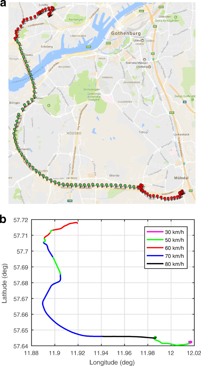
The route of the second scenario. In the top figure, the entries marked as green show the minor highway part (two lanes or more), while the ones in red are rural roads. The bottom figure shows the speed limits along the route
Resource for vehicle research laboratory: http://www.chalmers.se/en/researchinfrastructure/revere/Pages/default.aspx(2016).
URL: http://www.chalmers.se/vehprop(2017).

References
Nyberg P (2015) Evaluation, Generation, Transformation of Driving Cycles. Ph.D. thesis, Linköping University, Linköping.
Rexeis M, Quaritsch M, Hausberger S, Silberholz G, Kies A, Steven H, Goschütz M, Vermeulen R (2017) VECTO tool development: Completion of methodology to simulate heavy duty vehicles’ fuel consumption and CO2 emissions. DG CLIMA, Brussel. https://ec.europa.eu/clima/sites/clima/files/transport/vehicles/docs/sr7_lot4_final_report_en.pdf.
Eriksson L, Nielsen L (2014) Modeling and control of engines and drivelines. 1st edn, Wiley. http://common.books24x7.com.proxy.lib.chalmers.se/toc.aspx?bookid=63651.
Guzzella L, Sciarretta A (2013) Vehicle Propulsion Systems, 3rd edn. Springer, Heidelberg.
Edlund S, Fryk PO (2004) The Right Truck for the Job with Global Truck Application Descriptions In: SAE Technical Paper 2004-01-2645. https://doi.org/10.4271/2004-01-2645.
Pettersson P, Berglund S, Ryberg H, Karlsson G, Brusved L, Bjernetun J, Jacobson B (2016) Comparison of dual and single clutch transmission based on Global Transport Application mission profiles. Accepted in Int J Vehicle Design.
Nedělková Z, Lindroth P, Patriksson M, Strömberg AEfficient solution of many instances of a simulation-based optimization problem utilizing a partition of the decision space In: Annals of Operations Research 265, 93–118. https://doi.org/10.1007/s10479-017-2721-y.
Lindroth P (2011) Product Configuration from a Mathematical Optimization Perspective. Chalmers University of Technology. Ph.D. thesis. https://research.chalmers.se/publication/140022.
Vagg C, Brace CJ, Hari D, Akehurst S, Poxon J, Ash L (2013) Development and field trial of a driver assistance system to encourage eco-driving in light commercial vehicle fleets. IEEE Trans Intell Transp Syst 14(2):796–805. https://doi.org/10.1109/TITS.2013.2239642.
Dupuis M (2015) OpenDRIVE format specification, rev 1.4. H. VIRES Simulationstechnologie GmbH, Bad Aibling Germany. http://www.opendrive.org/docs/OpenDRIVEFormatSpecRev1.4H.pdf.
Various (2015) OpenCRG User manual. M. VIRES Simulationstechnologie GmbH, Bad Aibling. https://www.vires.com/opencrg/docs/OpenCRGUserManual.pdf.
Barlow T, Latham S, McCrae I, Boulter P (2009) A reference book of driving cycles for use in the measurement of road vehicle emissions. Tech. Rep. 3, TRL, Wokingham,Published project report PPR354.
Tutuianu M, Marotta A, Steven H, Ericsson E, Haniu T, Ichikawa N, Ishii H (2013) Development of a World-wide Worldwide harmonized Light duty driving Test Cycle (WLTC). Tech. Rep. UNECE Transport, UN Economic Commission for Europe, Sustainable Transport Division, Palais des Nations, CH-1211 Geneva 10. Informal document GRPE-68-03.
AB Volvo (2016) Predictive cruise control I-SEE. http://www.volvotrucks.us/powertrain/i-shift-transmission/i-see/. Accessed 01 Mar 2017.
Scania AB (2013) Spectacular fuel savings - Scania Opticruise with performance modes. https://www.scania.com/group/en/spectacular-fuel-savings-scania-opticruise-with-performance-modes/ Accessed 01 Mar 2017.
Daimler AG (2012) Predictive powertrain control - clever cruise control helps save fuel. http://media.daimler.com/marsMediaSite/en/instance/ko/Predictive-Powertrain-Control---Clever-cruise-control-helps-.xhtml?oid=9917205 Accessed 01 Mar 2017.
Torabi S, Wahde M (2017) Fuel consumption optimization of heavy-duty vehicles using genetic algorithms In: 2017 IEEE Congress on Evolutionary Computation (CEC), 29–36. https://doi.org/10.1109/CEC.2017.7969292.
Ghandriz T, Hellgren J, Islam M, Laine L, Jacobson B (2016) Optimization based design of heterogeneous truck fleet and electric propulsion In: Proceedings, ITSC, IEEE 19th international conference on intelligent transportation systems, 328–335.. IEEE, Red Hook. https://doi.org/10.1109/ITSC.2016.7795575.
Olofsson M, Pettersson J (2015) Parameterization and validation of road and driver behavior models for CarMaker simulations and transmission HIL-rig. Master’s thesis, Chalmers University of Technology,Göteborg.
Johannesson P, Podgórski K, Rychlik I (2017) Laplace distribution models for road topography and roughness In: Int J Vehicle Performance 3, 224–258. https://doi.org/10.1504/IJVP.2017.085032.
Speckert M, Dreißler K, Ruf N, Halfmann T, Polanski S (2014) The Virtual Measurement Campaign VMC concept - a methodology for georeferenced description and evaluation of environmental conditions for vehicle loads and energy efficiency In: Proceedings of the 3rd Commercial Vehicle Technology Symposium, 88–98.. University of Kaiserslauten, Kaiserslauten.
Pettersson P, Jacobson B, Berglund S (2016) Model for automatically shifted truck during operating cycle for prediction of longitudinal performance. Tech. Rep., Department of Applied Mechanics, Chalmers University of Technology, S-412 96, Goteborg̈. https://publications.lib.chalmers.se/publication/244540-model-for-automatically-shifted-truck-during-operating-cycle-for-prediction-of-longitudinal-performa.
Jacobson B (2016) Vehicle dynamics compendium. 1st edn. Chalmers university of technology, Göteborg.
Wong J (2008) Theory of ground vehicles. 4th edn. Wiley, Hoboken.
Contreras U, Li G, Foster C, Shabana A, Jayakumar P, Letherwood M (2013) Soil models and vehicle system dynamics In: Applied Mechanics reviews 65.apr, 040802–21. https://doi.org/10.1115/1.4024759.
Harnisch C, Lach B, Jakobs R, Troulis M, Nehls O (2005) A new tyre-soil interaction model for vehicle simulation on deformable ground In: Vehicle system dynamics 43.1, 384–394. https://doi.org/10.1080/00423110500139981.
Mechanical vibration – road surface profiles – reporting of measured data (1995) Standard. International Organization for Standardization, Geneva.
Johannesson P, Rychlik I (2016) Modelling roughness of road profiles on parallel tracks using roughness indicators In: International Journal of Vehicle Design 70.2, 183–210. https://doi.org/10.1504/IJVD.2016.074421. Accessed 12 Apr 2018.
Jin-qui Z, Zhi-zhao P, Lei Z, Yu Z (2013) A Review on Energy-Regenerative Suspension Systems for Vehicles In: Proceedings of the world congress on engineering 2013 Vol. 3, 1889–1892.. Newswood Limited/IAENG, Hongkong.
Green DW, Perry RH (2008) Perry’s chemical engineers’ handbook. 8th edn. McGraw-Hill, New York.
Elefteriadou L (2014) An introduction to traffic flow theory. 2014th ed. Springer, New York.
Ni D (2011) Multiscale modeling of traffic flow In: Mathematica Aeterna 1.1, 27–54.
NavmartHere traffic patterns. http://navmart.com/here-traffic-patterns/. Accessed 01 Mar 2017.
TomTom International B. V.If you can’t measure it, you can’t improve it. http://www.tomtommaps.com/en_us/traffic/. Accessed 01 Mar 2017.
Eriksson A (1997) Simulation based methods and tools for comparison of powertrain concepts. Licentiate thesis Chalmers University of Technology, Göteborg.
Karlsson M (2007) Load Modelling for Fatigue Assessment of Vehicles - a Statistical Approach, Ph.D. thesis, Chalmers University of Technology. Department of Mathematical Sciences, Chalmers University of Technology, Göteborg.
Reymond G, Kemeny A, Droulez J, Berthoz A (2001) Role of lateral acceleration in curve driving: driver model and experiments on a real vehicle and a driving simulator In: Human factors 43.3, 483–495.
Johnson L, Nedzesky AJ (2004) A comparative study of speed humps, speed slits and speed cushions. Tech. Rep. Annual meeting compendium, U.S. Department of Transportation Federal Highway Administration.
Chatzikomis CI, Spentzas KN (2009) A path-following driver model with longitudinal and lateral control of vehicle’s motion In: Forschung im Ingenieurwesen 73.4, 257. https://doi.org/10.1007/s10010-009-0112-5.
Berglund S (1999) Members, Modeling Complex Engines as Dynamic Powertrain. Chalmers University of Technology, Göteborg.
Acknowledgments
The authors would like to thank Dr Fredrik von Corswant and Mr Arpit Karsolia at the Revere lab for valuable help during the vehicle logging session.
This work is a part of the OCEAN-project, funded by the Swedish Energy Agency via FFI.
Author information
Authors and Affiliations
Contributions
The authors designed the format proposal together. PP performed the simulations and drafted the manuscript. LF and PP performed the experiment. All authors read and approved the final manuscript.
Corresponding author
Ethics declarations
Competing interests
The authors declare that they have no competing interests.
Publisher’s Note
Springer Nature remains neutral with regard to jurisdictional claims in published maps and institutional affiliations.
Rights and permissions
Open Access This article is distributed under the terms of the Creative Commons Attribution 4.0 International License(http://creativecommons.org/licenses/by/4.0/), which permits unrestricted use, distribution, and reproduction in any medium, provided you give appropriate credit to the original author(s) and the source, provide a link to the Creative Commons license, and indicate if changes were made.
About this article

Cite this article
Pettersson, P., Berglund, S., Jacobson, B. et al. A proposal for an operating cycle description format for road transport missions. Eur. Transp. Res. Rev. 10, 31 (2018). https://doi.org/10.1186/s12544-018-0298-4
Received:
Accepted:
Published:
DOI: https://doi.org/10.1186/s12544-018-0298-4