- Original Paper
- Open access
- Published:
Vehicle energy savings by optimizing road speed-sectioning
European Transport Research Review volume 12, Article number: 41 (2020)
Abstract
In a context of decreasing resources and of climate change, lowering road vehicles consumption is a key point to meet CO2 reduction requirements. In addition to car technological advances, eco-driving is part of the solution but the road infrastructure should ensure its development. This work aims to demonstrate that road energy demand and associated pollutant emissions can be reduced by working out minor optimization of road infrastructure itself. For this to happen, a simple eco-driving potential criterion is built upon infrastructure parameters such as slopes and sight distances. This criterion aims to detect Misplaced Speed-sectioning Positions (MSP) with regard to the Starting Point of Deceleration (SPD); with speed-sectioning being the succession of speed changes along a given route. An enhanced energy waste formulation is then developed to quantify the vehicles energy waste due to misplaced road-signs. Thirdly, a traffic simulation constitutes a framework for energy evaluation; considering a full flow of vehicles, based on real traffic data, and by modeling several driver behaviors. Simulation results show that a significant fuel reduction of up to 5.5% can be achieved locally, simply by moving a road sign, for rural areas and without degrading road safety.
1 Introduction
1.1 Energy context
According to the International Panel on Climate Change (IPCC) scenarios consistent with global warming below 1.5∘ C are needing a 15% reduction in transport sector final energy use by 2050 compared to 2015 [1]. Yet the same study underlines an annual increased of the transport sector emissions by 2.5% between 2010 and 2015, that accounted in 2014 for 28% of global final energy demand. New forecasts are always worse, global warming below 2∘ C appearing to be out of reach. The transport sector is particularly concerned with 80% of its energy needs relying on fossil fuels [2, 3].
Concretely the road transportation impact on climate change can be lowered by: encouraging eco-driving behaviors or limiting the use of car itself (Driver part), enhancing vehicle efficiency (Vehicle part), reducing the infrastructure-linked energy demand (Infrastructure part). This infrastructure part is generally less studied as a road energy mitigation mean since infrastructures are usually seen as an unchangeable constraint. However the present research proves that slight road infrastructure adaptation can lead to significant reduction of vehicle energy consumption.
The research is focused on energy reduction rather than direct emissions which are impacting climate change. However, currently almost all motorized vehicles are using oil. Electric vehicles are not in a significant amount, and in certain countries the electricity comes from coal, gas or oil. So there is a direct relation between oil use for road transportation and emissions. Reducing energy waste is directly contributing to emissions reduction and so to climate change mitigation.
1.2 Road energy mitigation
Limiting the use of car by modal shifts can lead to a high energy reduction, mainly in dense areas benefiting of bike lanes, buses, tramway. In contrary car dependency remains high outside the core of large cities [4, 5].
If not renouncing to use cars, drivers can still lower their energy consumption by adopting eco-driving behaviors [6–8], which could lead to reductions in fuel consumption and CO2 emissions ranging from 5% to 40% [9]. As an illustration an experimental study has concluded that eco-driving can lead to CO2 savings of 17% and 21% in gasoline and diesel engines, with a restrained increase of 7.5% in travel time [10]. Yet eco-driving can lead to over consumption by generating traffic speed spreading in specific situations [11].
Eco-routing is another mean for drivers to organize a trip with an energy optimization aim. In this field, managing vehicle speeds to avoid deceleration/stop at red lights results up to 19% energy savings [12]. The road profile parameter has been added in a study centered on drivers [13], facing the vehicle velocity profiles, with gains associated to accelerating on downhill slopes and slowing down on uphills slopes instead of driving at constant speed.
If considering vehicles, engine efficiency has been improved, but global efficiency has been limited by rising demand for Sport Utility Vehicles and comfort equipment as air conditioning or large tires [14].
Road as a variable to decrease energy demand in its use phase may be studied in the design stage, in order to compare projects [15], or, for a given project, to optimize the longitudinal profile [16]. However, these studies do not focus on gains achievable when roads have yet been build. For existent roads, some studies have linked infrastructures parameters to operating energy. For example in [17] road grade and turn radius have been found to have respective impacts of 18% and 37% on Operating Speed, which is the 85-th percentile of the speed distribution under free flow conditions). Variations of Operating Speed lead to the concept of Speed-Acceleration Joint Distribution (SAJD). SAJD changes in response to road grade have been discussed in [18], and as a result, the energy demanded by vehicles, defined as Vehicle Specific Power (VSP), is altered by road grades which condition the SAJD distribution. Energy variations of around 10% are associated to 4% grades.
1.3 Research methodology
In the framework of road energy mitigation, studies have mostly been focused on drivers and vehicles. Infrastructure impacts are more related to consequences of inadequate speed limits rather than on their optimization, and for road safety rather than energy efficiency.
Almost all decisions for design and exploitation of roads are related to safety and mobility efficiency. And it is a real and timely opportunity to add the energy savings to those criteria. If travel time can suffer a little, to the profit of climate change mitigation, safety can not. Therefore, the present methodology always proposes an extension of low speed zones to improve the adequacy between slopes, vehicle dynamics and speed sectioning. extension of the higher speed zones over lower speed zones is not an option.
On this basis a first study [19] demonstrated benefits of displacing a road sign position for improving eco-driving applicability in the adverse situation where vehicles have to decelerate on downhill situations.
This study was addressing the general issue that a speed-sectioning, defined as the succession of speed limitations by road signs, roundabouts, and crossings, is often impeding eco-driving, given the corresponding vehicle dynamics and road longitudinal profile (slopes). The present work extends this first study, by proposing evaluations of speed-sectioning in order to favor eco-driving in regards to vehicle dynamics, driver behaviors and road profiles.
The major novelty is to propose a comprehensive methodology to detect, optimize, and assess a speed sectioning in three steps. The first step is to propose a criterion usable by road managers to rapidly detect inconsistencies in speed-sectioning. The second step gives further information to road managers by quantifying the vehicles energy waste due to a given misplaced point of speed-sectioning, for a particular vehicle. The third step of our methodology involves a traffic simulation enabling an enhanced energy evaluation of new speed sectioning, while considering a full flow of vehicles, based on real traffic data, and modeling several driver behaviors.
Steps 1 and 2 are described in the next section. Experiments carried out in France and in Bosnia to extract road infrastructure data are presented in the third section. In the simulation section traffic is simulated in order to most closely determine potential energy gains. The fifth section displays significant results about the misplaced speed-sectioning detected in France and Bosnia-Herzegovina according to our three steps methodology.
2 Road speed-sectioning impact on vehicles consumption
2.1 Background
Regarding environmental and economical issues, more drivers are willing to eco-drive. However, there are some locations on their routes that prevent them to eco-drive. A class of these locations is considered in this work, for which drivers apprehend a speed-sectioning change without having the necessary distance to decelerate without braking strongly, which is contrary to eco-drive, since anticipation could have lead to lower beforehand speed and energy consumption. This class of locations will be called MSP for Misplaced Speed-sectioning Point locations in the following. These points are misplaced in an eco-driving meaning. Similarly the SPD position, which stands for Starting Point of Deceleration, is defined by the associated position where the driver apprehends the deceleration requirement and applies an effective command to comply with it.
Here, speed-sectioning is supposed to result of a road sign, among other road elements as roundabouts, crossings, speed bumps, …
The SPD position takes into account the driver reaction time, which is of the order of one or two seconds [20], with the associated traveled distance denoted dreac.
Figure 1 illustrates this concept of MSP. A transition between two constant-speed sections of a route is presented. The sectioning is represented by the vertical solid line at the MSP abscissa. Before this limit, the authorized speed is VSPD. After that, it becomes VMSP.

Ecodriving trajectories through a well- (dotted green) and poorly- (cyan) designed speed-sectioning
Cyan and green curves both represent the trajectories of an eco-driver, who releases the gas pedal as soon as she/he sees the speed limit sign, thus initiating its decelerating maneuver at the SPD point. In the green curve case the speed sign is ideally placed since the vehicle reaches it at the exact VMSP regulation speed. It is the configuration aimed by our optimization. On the contrary, in the cyan curve case, the driver, although being an eco-driver, has to apply mechanical braking while reaching the MSP point.
2.2 First level criterion for critical road speed-sectioning detection
In this part a criterion is developed to identify speed signs placed on locations which do not allow eco-driving. Energy losses associated to these detected misplaced signs (MSP locations) are then calculated as an evaluation tool for road managers.
On a given route, to detect if a speed sign is not consistent with eco-driving, vehicles dynamical situations are evaluated at the MSP and SPD predefined points (supposed to be misplaced). Between these two points the dissipated energy by rolling without braking nor accelerating, called natural deceleration, is compared with the energy to be dissipated to reach the regulatory speed at MSP, VMSP, from the speed of the vehicle at SPD, VSPD.
The energy to be removed for a given vehicle of mass m between the SPD and MSP points is the difference in mechanical energy:
Kinetic and potential energies to be erased are \(\Delta \text {Ek} = \frac {1}{2} \mathrm {m} \left (\mathrm {V_{SPD}^{2}} -\mathrm {V_{MSP}^{2}}\right)\) and ΔEp=mg(hSPD−hMSP) (J), with m (kg) the vehicle mass, hSPD and hMSP (m) the altitudes at SPD and MSP points and \(\mathrm {V_{SPD}^{2}}, \mathrm {V_{MSP}^{2}}\) the vehicle speeds (m/s) at the SPD and MSP points. In the following, speeds will be expressed in km/h by commodity, but calculation are done in m/s.
This difference in mechanical energy should have to be compensated by dissipating forces without mechanical braking as it will be detailed in the next section, but intrinsically, its amount is already a criterion since it is fixing the level of dissipating forces that will have to be worked out.
This first level criterion aims to be vehicle-independent for a convenient use by road managers. However dissipation forces are car-specific. They derive mainly from rolling and air resistance and are then linked to the weight, mg, directly for the rolling resistance and indirectly for the aerodynamic drag. Moreover by noticing that this energy is an integration of power along the maneuver distance dman, a dimensionless criterion is proposed χEASM (EASM = Energy Alert Speed Management):
Where dman (m) is the driver maneuvering distance, which separates SPD and MSP points.
This distance is active through a logarithm function because an important part of the energy dissipation is the integration of the aerodynamic drag power which decreases as the vehicle decelerates along the maneuver distance. The logarithm has the same feature: its first derivative is positive and its second is negative.
This criterion summarizes thus the energy interpretation. By developing this equation, the criterion is independent of vehicle parameters:
Road managers have therefore a convenient criterion to evaluate rapidly the speed transitions of their networks and to detect easily transitions where χEASM is important and for which eco-driving is consequently not favored. After having detected these transitions they could move the speed limiting sign in a nearby site with a better eco-driving potential i.e. a better visibility of the sign or without a road slope. Validation of the new sign position is done by calculation of the criterion at this new position.
2.3 Enhanced energy criterion to evaluate route speed-sectioning
The simple criterion χEASM defined in the previous section is improved here towards an energy waste formulation denoted \(\mathcal {EW}_{MSP}\) which takes into account more explicitly the vehicle dissipation forces. This energy waste \(\mathcal {EW}_{MSP}\) associated to the misplaced speed sign will be determined in this section in terms of energy for each single car, before being determined for a traffic on a road in a dedicated section by using traffic simulation. It is an energy waste in the sense that this amount of energy could have been save with an optimal position of the speed sign, according to the slope and the vehicle dynamics, driver behavior.
Again, natural deceleration from VSPD to VMSP is considered.
The vehicle is modeled by a point model to which are applied the following forces (Fig. 2):
aerodynamic drag: \(\frac {1}{2} \rho S C_{x} \mathrm {w_{a}}^{2}\), with ρ air density (kg/mş), S front vehicle area (mš), Cx drag forces coefficient, wa apparent wind (m/s, assumed to be equal to the v speed)
Fig. 2 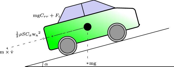
Vehicle model
rolling resistance: mgCrr, with m vehicle mass (kg), g acceleration of gravity (m/sš), Crr coefficient of rolling resistance,
internal forces of the vehicle : Fi which sums frictions and motor resistance (N),
the gravity forces: mg sin(αr) (N), with αr angle of slope in radian.

The following equation is obtained
By integrating this ordinary differential equation, the \(\mathcal {EW}_{MSP}\) energy waste is:
\(\mathcal {EW}_{MSP}\) represents the energy to be dissipated by the brake system. It is the difference between the total energy at the speed v(tf) (m/s) and that of the target speed VMSP (Fig. 1). v(tf) is the speed at which the vehicle arrives at MSP. The analytical calculus of v(tf) is detailed in Appendix A.
By considering this energy gain potential, a road manager can displace the MSP sign, by the dmanopti distance (m) which is the travelled distance by a vehicle in natural deceleration from VSPD to VMSP (distance computed analytically in Appendix A). By doing that, the speed sectioning is optimized for a given vehicle driven in a eco-driving manner.
It is in fact the optimal distance from the MSP point where the eco-driver has to start his deceleration (SPD), as displayed by the green dotted curve on Fig. 1.
In the next section, experiments are presented in order to support this theoretical analysis.
3 Experimental evaluation of a route speed-sectioning
Criterion and energy waste validation experiments have been done on two road routes, in Bosnia-Herzegovina and France. These experiments will provide as well some input for the simulation part of this methodology. The vehicles used for the experiments are instrumented in order to get the visibility distance and the geometric configuration of the road.
These experiments, and the associated results of this paper, are focused on non urban roads. Indeed, there is a high potential of energy economy, with considerable speed reductions and a large traffic proportion, compared to urban regions. Moreover, in urban areas the complexity of the crossings, lanes dispositions, succession of equipment (roundabouts, lights, dedicated lanes) and modes (cycles, pedestrians) are limiting the applicability of the proposed methodology, both for efficiency and safety aspects. Urban environment is even limiting the realization of experiments with good safety and repeatability levels.
However, experimentation contribution to models could allow the afterwards application of the methodology in urban areas, while adding safety and mobility parameters.
3.1 Experimental setup
Both test campaigns consisted of:
browsing the road network to identify locations where a speed-sectioning change impedes eco-driving. In the usual case such a location is the emplacement of a road limiting sign placed in a strong descent, for which drivers have to apply mechanical braking, instead of simply decelerating,
driving through these locations with a test vehicle, while recording vehicle route with a non-differential NMEA GPS (acquisition frequency of 1 Hertz; punctual imprecision smoothed by signal interpolation),
telling to the driver to drive at the allowed speed VSPD, to decelerate as soon as she/he sees the speed sign (SPD point), and to brake if she/he goes past the sign if her/his speed is in excess (> VMSP), in order to comply with road traffic regulations. This driving procedure aims to verify onsite if speed sign is misplaced, although speed evolution is not processed furthermore by our models. These models need only the relative 3D positions of SPD and MSP locations. This driving procedure is also the closest to classical eco-driving rules.
taking two geo-tagged pictures of the scene from a high resolution webcam: one when the driver is perceiving the speed limiting sign, one when she/he reaches effectively this sign. Geo-tagging is implemented on a linux-based laptop with the help of a time correlation procedure between the gps device and the image capture device, both of them being time-synchronized by the computer,
recording continuously the following signals: longitudinal wind speed by a roof anemometer, Bus-Can instantaneous fuel consumption, central inertia unit angles, engine throttle angle. These signals are processed to identify the car specific parameters. This information is not required to compute the simple criterion χEASM but are valuable to compute the \(\mathcal {EW}_{MSP}\) waste according to Eq. 5. This equation is based on Eq. 11, including vehicle parameter: a and c. These parameters are identified by using dedicated experiments. When coasting, the observed deceleration is compared with the deceleration computed with Eq. 11. The parameters are optimized so that the computed deceleration is as close as possible to the measured deceleration.
3.2 Experiment in France
As detailed in [19], experiments have been done while crossing the French small village "La Brossière". The village is represented in grey on the map (Fig. 3) and the blue elevation graph gives first information on the fact that this village is in a "bowl" situation: both of the two village entrances present rather high downhill slope. The yellow dot on the blue route represents the southern village entrance.

Experimental car reaching the limiting speed sign at "La Brossière"
For this situation case, positions of viewing and passing the road sign are considered.
The distance between the two positions is of 300 meters;
The respective altitudes are 189.7 m and 178.7 m (difference of 11 meters);
The speed has to be reduced to 50 km/h from 90 km/h (reduction of 11.11 m/s).
The test vehicle is a mid-size passenger car, which weighs 1064 kg, has an average consumption of 4.6 l/100km, an aerodynamic frontal surface of 2.06 m2 and a Cx-air penetration coefficient of 0.30.
This case is then associated to a high potential energy equal to 49.9% of the kinetic energy, both energy having to be cut down for decelerating appropriately. Alert criterion is then unsurprisingly high (given by Eq.2 and Eq. 3).
High values of criterion and energy waste will be associated with this situation requiring a strong deceleration. These results will be presented in the following global result section.
3.3 Experiment in Bosnia-Herzegovina
Complementary experiments have been carried out in Bosnia-Herzegovina to get data in order to extend the applicability of our methodology to several countries, road managements and land topography. Road experiments have been done over 140 km, on the M-5 (Mostarsko raskrsce-Kiseljak-Busovaca) and M-18 roads (Vogosca-Olovo-Stupari). 9 road-signs have been found to be problematic in the sense of eco-driving capabilities. Suspected "negative" example of a sign layout has been found at the exit of the village "Kobiljaca", on the R442; M-5 and in the south-north direction. At this point drivers have to decelerate from 80 km/h to 40 km/h without having a sufficient maneuver distance. Braking is necessary, whereas an implantation of an advance warning would have allow to "eco-drive" (coasting from the warning sign to the speed limiting sign enabling to reach the speed limitation without using mechanical braking). Here the constraint is the curve which limits the sign visibility, on contrary to the descent in the French case which was limiting the decelerating capability.
In this experiment an another passenger car has been used. It has an average fuel consumption of 6.1 l/100km, an aerodynamic frontal surface of 2.19 m2 and a Cx-air penetration coefficient of 0.32. The two cars used for experiments in France and Bosnia are quite similar which is an advantage to compare encountered test cases in both countries.
For this situation case, just after a turn, positions of viewing and passing the road sign are considered.
The distance between the two positions is of 50 meters;
The respective altitudes are 625 m and 629 m (difference of 4 meters);
The speed has to be reduced from 80 km/h to 40 km/h (reduction of 11.11 m/s).
This case is then associated to a low potential energy, high kinetic energy variations and a short maneuver distance. It will be seen in the following Section 5 that will lead to high alert criterion and energy waste.
Only 50 meters available for the deceleration maneuver could be seen as a faulty road management, but road sign has probably been implemented here to protect nearby population, without having other design choice, since associated mountainous terrain result in frequent and marked curves, local roads being strongly adjusted to local ground conditions [21]. So, this implantation is constrained by the mountainous environment, it is acceptable in a road safety point of view, with an acceptable required deceleration rate, but it is impeding eco-driving.
4 Speed-sectioning energy waste evaluation by simulating driving behaviour
This section aims to evaluate the energy waste of the previous detected critical speed-sectioning in the Bosnian experiment. In order to represent the energy impact of the original and modified speed-sectioning we have choose to run traffic flow simulations, with real local traffic data, real road geometry and with realistic vehicles and drivers models.
Synchro Trafficware constitutes the simulation framework. It is based on HCM2010 methodology [22] and its has about one hundred parameters which take into account our experimental conditions on road geometry, traffic structure (vehicles) and driver behaviors. This simulation framework is designed to be flexible enough that we could correctly calibrate the network and vehicle/drivers diversity to match the local real world conditions at a reasonably accurate level.
4.1 Drivers modeling
Modeling the driving conditions is definitely not an exact science. Experiments have shown that speed-sectioning modifications could lower energy consumption for drivers who are following a strict eco-driving strategy: drive at the restricted speed, decelerate as soon as speed limit is perceived, brake only if restricted speed is exceeded.
In real world, driving behaviors are varied in a very complex manner and an evaluation of the energy waste of a speed-sectioning should embrace that variety. However, only 4 types of drivers would be considered in the following, due to modeling complexity feasibility and to the lack of information on the behaviours of drivers in the considered traffic:
Type 1 (aggressive) where the deceleration varies from 1.4 to 3.0m/ s2,
Type 2 (defensive e.g-elderly drivers) where the deceleration varies from 0.7 to 1.0m/ s2,
Type 3 (eco-drivers) where the deceleration varies from 0.3 to 0.4m/ s2 following the study [23],
Type 4 (combination of all types (30% of type 1, 40% type 2, 30%type 3)) in accordance to their manoeuvre distance.
Figure 4 illustrates the behavior of two types of non eco-driver in comparison with the trajectory of an idealized eco-driver while approaching a speed sectioning. The blue curve is the simplified trajectory of a vehicle driven by a type 1 driver. The driver speed, \(\mathrm {V_{SPD}^{a}}\) is slightly above the authorized speed V1. A speed factor is then defined from this speed difference, with \(\mathrm {V_{SPD}^{a}}\) equal to V1 multiplied by the speed factor. This speed is in fact directly altered by the speed factor (higher than 1). After seeing the speed limiting sign, the driver will brake mechanically with the highest deceleration of the driver type until reaching his new speed target, altered by the speed factor.

Different trajectories of passage through a sectioning from different drivers
The grey curve represents the simplified trajectory of the type 2 driver who will drive slower, at the speed \(\mathrm {V_{SPD}^{o}}\), than the V1 regulatory speed and with a longer reaction delay. The deceleration is still important because she/he wants to comply with the speed limit although its longer reaction delay. This grey curve is mostly representative of old drivers. In that case the speed factor is lower than 1.
The cyan curve represents the idealized eco-driver (type 3), who will release the gas pedal as soon as she/he sees the speed limiting sign. Its deceleration is the smallest of the driver types. The speed of the eco-driver is consistent with the regulatory speed. At last, for that case the speed factor is strictly equal to 1.
When a driver encounters a change in the speed-sectioning, the situation constitutes an "analyse/action event" with the following parameters:
entry parameters: initial speed, local slope and turn, visibility,
action parameters: speed sign detection, starting position of decelerating, braking duration and intensity choices,
consequences parameters: be at the designed speed before reaching the speed sign or not, necessity of braking or not.
The simulation framework models the driver with a proportional speed law i.e the cruise speed of the driver is proportional to the regulatory speed. Therefore in order to simulate the parameters of the complex defined "analyse/action event" it has been chosen to compensate shifts in decelerating positions by a speed factor parameter.
Statistically, speed factor can be used by traffic models to compensate fine real variability in driving behaviors, variations in initial speed and deceleration rates compensating variations in instant decision of decelerating and braking.
At last, types of drivers will be associated to several types of vehicles in the simulations, without specific link between types of drivers and vehicles.
4.2 Speed-sectioning modeling
In order to evaluate speed-sectioning optimization within the simulation framework the three following scenarios are taken into account:
Scenario 1: in the simulation the speed-sectioning changing point is exactly at the same location as in the experimental situation,
Scenario 2: speed-sectioning changing point is implanted in the simulation in an upstream optimized placement for eco-driving,
Scenario 3: an advance warning is simulated by adding an intermediate speed reduction upstream in the simulated road section (80 km/h to 60 km/h then to 40 km/h), thus enhancing eco-driving opportunity for most driver types.
4.3 Model inputs: road and traffic data
The simulation is done with a flow of varied vehicles and it is based on the experiment conducted in Bosnia-Herzegovina. Considered experimental road is a bidirectional with very few intersections with local unpaved roads that will be neglected.
The analyzed trajectory is the same as the one used in experiment part (Kobiljaca/ R442/ M-5). Associated traffic data has been provided by the road survey service of the Federation of Bosnia-Herzegovina. This road section has an average annual daily traffic (AADT) of 12,452 vehicles. Data are provided by using STERELA counters and QLD-6CX i QLTC 10 (marked as yellow and purple triangles on the map, Fig. 5).

Map of the Main Roads Network of the FBIH with special reference to the 523 and 585 counters
4.4 Set up of the simulation traffic flow
OpenStreetMap is used to apprehend the simulated road environment, enriched with the Bosnian case experimental data (Fig. 6). Route length is of 1189 meters and speed-sectioning is defined by the effective positions of road signs. So each simulated segment has its own speed limitation regarding to experimental data. So, speed limits used in the simulation model are the same as in the real-life Bosnian experiments.

Road calibration on trafficware platform
The daily distribution of the traffic used for the simulations is given in Table 1 according to the following vehicle classes: A1-motorcycle; A2-personal car; A3-private car with trailer; A4-van with or without trailer; B1-small truck; B2-medium truck; B3-heavy freight vehicle; B4-heavy freight vehicle with trailer; C1-Bus. There is a large predominance of the personal car class (A2).
Values of speed factor and deceleration rates are fixed for the four simulated types of drivers (Table 2).
As indicated previously, speed factor aims to take into account a sufficient variety of driving behaviors facing the evaluation gain of speed-sectioning optimisation. It allows for the concerned driver to adapt to the current link speed by this factor, which has a range of variation from 0.70 to 1.35. It alters directly the road design speed.
4.5 Simulation running conditions
The micro-traffic simulation has been run with combinations of measured traffic, simulated drivers and measured road infrastructure. Drivers are apprehending road geometry and speed restrictions and then control vehicles.
Vehicles dynamics depends on drivers commands, including individuals speed factors and deceleration, on road gradient and turns, and of course on particular vehicle characteristics. Moreover each vehicle is interacting with others in case of non-free flow conditions. As an example the interaction between different vehicles-drivers couples is shown in Fig. 7.

Example of the routes followed by different types of vehicles
In the general case of constrained traffic, the traffic flow simulation relies on the following general flow equation:
Where: q - flow (vehicles/hour), v - speed (kilometers/hour), k - density (vehicles/kilometer).
Simulations are conforming to HCM2010 equations and regulations [22].
However, in adverse situation with misplaced speed signs or regulations, the traffic simulation is able to point out traffic congestion, as it can be seen on Fig. 8 where average speeds are traced.

Segment of our route and representative average speeds
In the next section, simulations will help to quantify the impact of speed section’s alterations on traffic fluidity and fuel consumption. Within each simulation step, fuel consumption is determined for the vehicle fleet displacements (car, truck, or bus) over the whole calculation area (one kilometer long). In the retained simulation framework fuel models are derived from both empirical studies and theoretical equations. Final form of the consumption model used in this work is of:
where:
Fi = fuel consumed on link i, in liters per hour;
TTi = total travel in veh-km per hour;
TDi = total delay in veh-hr per hour;
TSi = total stops in vph; and
Kij = model coefficients which are functions of cruise speed (Vi) on each link i.
where Ajk are regression coefficients.
Fuel consumption expression is given here in its general form, however in practice it takes into account each vehicle characterized by its class, its dynamics and associated driver behavior.
5 Results
5.1 Energy waste: results for a single vehicle
Table 3 summarizes the experimental conditions in France and Bosnia and presents the speed-sectioning analysis results according to the Section 2 equations. In the French experimental case, the vehicle changes speed from 90 km/h to 50 km/h over 300m on a downhill road: the altitude variation is from 190m to 179m. The value of the Energy Alert Speed Management criterion, χEASM, is 13.3. The energy waste of the sign is 204 kJ.
In the Bosnian experimental case, the vehicle goes from a speed of 80 to 40 km/h over 50m however a road uphill is present: the altitude variation is from 625 to 629m. The criterion χEASM is 8.8. The energy waste of the sign is 199 kJ. The table third line is an example of a normal speed-sectioning with a speed of 80 to 50 km/h on a flat road.
The experiments in France and Bosnia were indeed carried out on roads with poorly designed speed-sectionings, which are black spots from the point of view of energy consumption. The energy dissipated in the brakes is 48% higher on these black spots than in the typical case: 138 kJ in the normal case, 199 and 204 kJ on Misplaced Speed-sectioning Positions. The criterion, χEASM, is higher on these black spots than in the normal cases: 6.7 in the normal case against 7.8 and 13.3 for the black spots cases.
The experiment in France represents a situation where the speed limiting sign is at the bottom of a descent. In Bosnia, the driver is surprised by the speed limiting sign because of a curve that masks the panel. In the first case, the mechanical energy to be dissipated is greater than in the second case. In Bosnia, it is the manoeuvre distance that is shorter than in France. In both cases, the energy to dissipate in the brakes, \(\mathcal {EW}_{MSP}{}\) is about the same. The criterion, χEASM, is different between the two experiments (7.8 for Bosnia, 13.3 for France) when they should be close. This criterion is based only on infrastructure parameters. In this particular case, this is less accurate than the waste associated to the panel, \(\mathcal {EW}_{MSP}{}\), which takes more into account the vehicle characteristics.
5.2 Results with traffic simulation
Beyond the methodology validation with isolated passenger cars, this section aims to evaluate energy waste due to a misplaced sign over a route and for various types of vehicles and driver behaviors.
A set of simulations has been carried out in order to evaluate the mean fuel consumption over a one kilometer section, for three speed-sectioning configuration and four driver types. Results are presented in Fig. 9. The X axis represents different types of drivers according to Table 2. The Y axis is the fuel consumption on defined route in a simulation of 10 minutes defined by the traffic data presented in Table 1. Inside the one kilometer section of simulation, there is only one speed change, from 80km/h to 40km/h. The three scenarios are differing only by the longitudinal position of the corresponding speed change sign as defined in Section 4.2.

Fuel consumption for 3 scenarios and 4 driver types over the simulation section
The results underline the specificity of our three scenarios. The main difference between the three scenarios on Fig. 9 is shown for the type 3 driver. This is explained by the fact that the actual infrastructure does not allow eco-driving. On the other hand, the other two scenarios allow eco-drivers to apply eco-driving rules, with a 5% gain on fuel consumption with the scenario 2 (14,4 l) compared to the scenario 1 (15,1 l) by optimizing the placement of the speed limiting sign, and 5.5% with the scenario 3 (14,3 l) by adding an advance warning sign.
These results are important as an improvement to an ecological potential of road infrastructure without lowering safety standards.
6 Discussion
6.1 Result analysis
As expected, an eco-driving friendly infrastructure does not reduce significantly fuel consumption for drivers who do not have such an eco-driving behavior. On Fig. 9, the fuel consumption of the driver types 1,2,4 is about the same between the initial speed-sectioning (Scenario 1) and the optimized speed-sectioning (Scenario 2) and the initial speed-sectioning with advance warning signs (Scenario 3). The objective of the scenario 3 was to force the trajectory of the normal drivers to become a soft trajectory, near to an eco-driving trajectory. This objective is not reached for non eco-driving drivers. The reason is that the drivers brake mechanically even along this soft trajectory. The conclusion is that gains are becoming increasingly important as the number of eco-driver increases.
6.2 Limits and hypotheses
-
We affirm that the criterion, χEASM is practical for the manager but the calculation of this criterion requires knowing the manoeuvre distance. In this work, we experimentally evaluated this one, which may be too complicated for the manager of a large road network. This experimental step can be avoided by using road design standards and rule-book on guidance for design, building, maintenance and supervision of the roads of each country as i.e [24] and [25].
From that, the distance Lz to decrease the speed to the speed sign is calculated according to:
$$ L_{z} = (V_{p}^{2} - V_{k}^{2})/ 26 \times (a_{z} + 0.1 \times s_{i}) $$(9)where Vp represents the initial speed and Vk is the final speed, az (m/ s2) is the natural deceleration value linked to usual friction coefficients, and si is the level of the longitudinal slope.
Assuming that this distance is verified, the manager has all the data to calculate χEASM without conducting the experimental part.
-
The simulation model has potential to assess the traffic locally on a defined route, however it has also some disadvantages. Driving behavior is modeled by automatized base-acceleration phases (speed adaptation factor), without the perception value of a human driver. We can say that even by adjusting the type of the driver, deceleration and acceleration phases does not represent accurately human successive driving processes. This weak point is addressed by our ongoing research.
-
Nevertheless simulations show that fuel consumption gains are significant (5.5%) for eco-drivers while being inexpensive for the infrastructure manager, because it is enough just to displace a speed limiting sign. A risk for the manager is that displacing a speed sign may cause congestion. This can increase greenhouse gas emissions contrary to our goal. Traffic simulations are then useful for assessing this undesirable effect.
-
Simulation results may underestimate actual fuel savings. Indeed simulation’s route length can not be shorter than one kilometer, albeit in real world there can be two or three points of speed-sectioning to be optimized in such a one kilometer length. So, in dense areas, optimizing speed-sectioning could lead to somewhat twice the previously estimated fuel savings.
-
At last, based on the research of [26] where a model of number of replications is explained and needed in a micro-traffic simulation to obtain reliable results, we checked that the number of replications was sufficient: we obtained the same results every time, conducted for each type of driver, because of the environment of trafficware model already does certain number of MOE (measure of effectiveness) for each simulation as we calibrated, and validated the speed factor of each type of driver, the starting point of each vehicle and the measuring period.
6.3 Applicability
The frequency of misplaced panels depends on various factors: geography, traffic sign norms, regulations... Resulting gains according to the displacement of a misplaced panel depends also of numerous variables: traffic, percentage of ecodrivers, compliance with the regulation. In Bosnia, we detected 9 misplaced panels over 140 km. In France, we detected 8 panels over 100 km of secondary roads. However, this frequency has decreased recently as the legal speed on these roads has been managed from 90 km/h to 80 km/h. Despite this variability, the most fruitful result should be reached for secondary roads in rural and mountainous area. In the other hand, our methodology should not bring significant improvements to highways because slopes and turns are moderated and visibility distances are higher.
7 Conclusion
A three-step methodology is developed in this work in order to provide progressive means of road energy demand reduction. This methodology is dedicated to road managers since it is focused on optimization of route speed-sectioning, which consists of the succession of limiting speeds along a given route. Indeed, some misplaced speed changing points do not allow drivers to eco-drive and improvement can be achieved by simple speed-sectioning modifications.
The first step is to propose a criterion, χEASM, rapidly usable by road managers to detect these points, named Misplaced Speed-sectioning Position (MSP), in relation to the Starting Deceleration Point (SDP) of approaching vehicles and road characteristics as slopes and turns. The second step yields further information to road managers by quantifying the energy waste due to a MSP-type speed changes. As the third step, a traffic flow simulation has constituted the frame of an enhanced energy assessment, while considering a full flow of vehicles, based on real traffic data, and by modeling several driver behaviors. Experiments have been conducted in France and Bosnia to demonstrate the applicability of this theoretical analysis. Simulation results show that a significant fuel reduction, up to 5.5% for eco-drivers can be achieved by simply displacing a speed limiting sign.
The criterion and the energy waste quantification are intrinsically applicable on every road, but the dense environment as can be found in cities and peri-urban areas are limiting their applicability, since crossings, equipment, other modes flows should require more parameters. The safety is more difficult to take into account in the dynamical model than in section without crossings and multiple modes (pedestrians, bicycles, dedicated lanes,...). However, a finer model, able to model parallel and perpendicular flows of various modes, each following different mobility rules. Such optimization are existing for energy sparing with the synchronization of green lights, but the present work, which associates slopes, allowed speeds and vehicle dynamics could be profitable in hilly cities.
Choice has been taken to apply the methodology on rural roads, and to use the simulation to state on the achievable fuel reductions for a large panel of vehicles including heavy vehicles. An ongoing research is focusing on the optimisation of a rural road speed-sectioning and for a longer route. In a future step, this optimisation process could be integrate in a microscale and multi-mode traffic and safety model.
As a current application, for rural areas, this efficient methodology, validated on real data, is inexpensive to implement and is proposed to managers in order to make their infrastructures more eco-driving friendly. Furthermore, authors of road guidelines can benefit from our methodology in order to improve road-sign placement rules.
Moreover, a pacification of the general traffic, by ensuring eco-driving potential of roads, is susceptible to improve the overall road safety, by tempering abrupt driving behaviors. The link of this methodology application to the accident rate remains to be quantify, but overall safety should be improved in the simpler situation of rural areas.
8 Appendix A
8.1 Computation of the panel energy waste \(\mathcal {EW}_{MSP}\) and the optimal position of the panel
In this annex, the computation of the panel energy waste is described. We restarted from ordinary differential Eq. 4
And so:
with \(a=-\left (\frac {1}{2} \rho C_{x} S_{x}\right)/\mathrm {m}\) and c=−g(Crr+ sin(α))−Fi/m
The solution of this differential equation provides the trajectory, i.e. the position of the vehicle and its speed as a function of time.
In the case of the simple, but usual, configuration without variation in slope, these calculations can be done analytically. It is then possible to calculate very quickly the energy waste due to a misplaced speed sign. For more complex spatial configurations digital computations are needed.
The analytical solution of ordinary differential Eq. 11 is:
with \(B=\sqrt {c/a}, A=\sqrt {ac}, K=-\arctan {\left (\mathrm {V_{SPD}}/B\right)}/A\).
The analytical calculation of the travelled position x as a function of time:
with E=1/|a|.
By setting the boundary condition x(t)=dman and by inverting Eq. 13, it yields that the time tf taken by the vehicle to travel the distance dman is given by the following equation.
The energy waste of the misplaced speed sign \(\mathcal {EW}_{MSP}\) is as following:
\(\mathcal {EW}_{MSP}\) represents the energy to be dissipated by the brake system.
Then the road manager could move the speed limiting sign. In order to help her/him to treat this MSP, the distance travelled by a vehicle from VSPD to VMSP without applying traction force nor mechanically braking is computed analytically in the following and is noted, dmanopti. The starting point of this distance is called Optimal SPD. Both are presented on Fig. 1 where the dotted green curve is the ideal trajectory of an eco-driver. By using warning sign or speed limiting sign, the road manager has to encourage drivers to follow this trajectory.
First, the time td required for this deceleration is computed by inverting Eq. 12 with v(t)=VMSP:
And the solution provided by the Eq. 12 is presented as:
dmanopti is the optimal distance from the MSP where the eco-driver has to start his deceleration as displayed on the Fig. 1. It gives directly the Optimal Starting Point of Deceleration (DSP) and furthermore the optimal position of panel knowing the visibility distance.
Availability of data and materials
Not applicable.
References
Rogelj, J, Shindell, D, Jiang, K, Fifita, S, Forster, P, Ginzburg, V, Handa, C, Kheshgi, H, et al. (2018). Chapter 2: Mitigation Pathways Compatible with 1.5 ∘C in the Context of Sustainable Development. In Global Warming of 1.5∘C an IPCC Special Report on the Impacts of Global Warming of 1.5∘C Above Pre-industrial Levels and Related Global Greenhouse Gas Emission Pathways, in the Context of Strengthening the Global Response to the Threat of Climate Change. Intergovernmental Panel on Climate Change.
de Coninck, H., Revi, A., Babiker, M., Bertoldi, P., Buckeridge, M., Cartwright, A., Dong, W., Ford, J., Fuss, S., Hourcade, J., Ley, D., Mechler, R., Newman, P., Revokatova, A., Schultz, S., Steg, L., Sugiyama, T. (2018). Strengthening and Implementing the Global Response, Chap. 4, (pp. 313–443). IPCC: In Press.
Santos, G. (2017). Road transport and co2 emissions: What are the challenges?Transport Policy, 59, 71–74.
Gao, Y., Kenworthy, J.R., Newman, P., Gao, W. (2018). 2.2 - Transport and Mobility Trends in Beijing and Shanghai: Implications for Urban Passenger Transport Energy Transitions Worldwide, Second edn., (pp. 205–223). 978-0-08-102074-6: Elsevier.
Belton Chevallier, L., Motte-Baumvol, B., Fol, S., Jouffe, Y. (2018). Coping with the costs of car dependency: A system of expedients used by low-income households on the outskirts of Dijon and Paris. Transport Policy, 65(C), 79–88.
Barla, P., Gilbert-Gonthier, M., Castro, M.A.L., Miranda-Moreno, L. (2017). Eco-driving training and fuel consumption: Impact, heterogeneity and sustainability. Energy Economics, 62, 187–194.
Huang, Y., Ng, E.C.Y., Zhou, J.L., Surawski, N.C., Chan, E.F.C., Hong, G. (2018). Eco-driving technology for sustainable road transport: A review. Renewable and Sustainable Energy Reviews, 93, 596–609.
Sivak, M., & Schoettle, B. (2012). Eco-driving: Strategic, tactical, and operational decisions of the driver that influence vehicle fuel economy. Transport Policy, 22(C), 96–99.
Alam, M.S., & McNabola, A. (2014). A critical review and assessment of eco-driving policy & technology: Benefits & limitations. Transport Policy, 35, 42–49.
Juan, C., Marta, G., Yang, W., Andrés, M. (2017). Green eco-driving effects in non-congested cities. Sustainability, 10(1), 28.
Qian, G., & Chung, E. (2011). Evaluating effects of eco-driving at traffic intersections based on traffic micro-simulation. In Australasian Transport Research Forum 2011 Proceedings, (pp. 1–11).
Zeng, X., & Wang, J. (2018). Globally energy-optimal speed planning for road vehicles on a given route. Transportation Research Part C: Emerging Technologies, 93, 148–160.
Ozatay, E., Ozguner, U., Michelini, J., Filev, D. (2014). Analytical solution to the minimum energy consumption based velocity profile optimization problem with variable road grade. IFAC Proceedings Volumes (IFAC-PapersOnline), 19, 7541–7546.
Weber, C., Sundvor, I., Figenbaum, E. (2019). Comparison of regulated emission factors of euro 6 ldv in nordic temperatures and cold start conditions: Diesel- and gasoline direct-injection. Atmospheric Environment, 206, 208–217.
Luin, B., Petelin, S., Al Mansour, F. (2017). Modeling the impact of road network configuration on vehicle energy consumption. Energy, 137, 260–271.
Vandanjon, P.-O., Vinot, E., Cerezo, V., Coiret, A., Dauvergne, M., Bouteldja, M. (2019). Longitudinal profile optimization for roads within an eco-design framework. Transportation Research Part D: Transport and Environment, 67, 642–658.
Praticò, F., & Giunta, M. (2012). Modeling operating speed of two lane rural roads. Procedia - Social and Behavioral Sciences, 53, 665–672.
Liu, H., Rodgers, M.O., Guensler, R. (2019). Impact of road grade on vehicle speed-acceleration distribution, emissions and dispersion modeling on freeways. Transportation Research Part D: Transport and Environment, 69, 107–122.
Coiret, A., Vandanjon, P.-O., Cuervo–Tuero, A. (2016). Ecodriving potentiality assessment of road infrastructures according to the adequacy between infrastructure slopes and speeds limits. In Cetra2016 – 4th International Conference on Road and Rail Infrastructure, (pp. 589–595).
AASHTO (2001). A policy on geometric design of highway and streets. Technical report.
Gaca, S., & Kiec, M. (2016). Speed management for local and regional rural roads. Transportation Research Procedia, 14, 4170–4179. Transport Research Arena TRA2016.
Highway Capacity Manual 2010. (2010). Transportation Research Board of the National Academies. Washington, D.C.
Cantisani, G., Serrone, G.D., Biagio, G.D. (2018). Calibration and validation of and results from a micro-simulation model to explore drivers’ actual use of acceleration lanes. Simulation Modelling Practice and Theory, 89, 82–99.
Association of State Highway & Transportation Officials. (2020). Guide Specifications for Highway Construction, 10th Edition.
Roads of federation of B&H. (2005). Guidelines for design building maintenance and supervision of roads. Technical report. Sarajevo-Banja Luka: University of Ljubljana and DD Consulting and Engineering.
Wilco, B. (2004). A note on the number of replication runs in stochastic traffic simulation models. working paper ctr2004:01. Technical report, Centre for Traffic Simulation, Royal Institute of Technology, Stockholm, Sweden., www.ctr.kth.se/publikationer/ctr2004_01.pdf.
Acknowledgements
We would like to thank the ’Roads of the Federation of B&H’ company for their assistance with the collection of our data for the simulation part.
Funding
Not applicable.
Author information
Authors and Affiliations
Contributions
All contributing authors are cited in first page. The author(s) read and approved the final manuscript.
Corresponding author
Ethics declarations
Competing interests
The authors declare that they have no competing interests.
Additional information
Publisher’s Note
Springer Nature remains neutral with regard to jurisdictional claims in published maps and institutional affiliations.
Rights and permissions
Open Access This article is licensed under a Creative Commons Attribution 4.0 International License, which permits use, sharing, adaptation, distribution and reproduction in any medium or format, as long as you give appropriate credit to the original author(s) and the source, provide a link to the Creative Commons licence, and indicate if changes were made. The images or other third party material in this article are included in the article’s Creative Commons licence, unless indicated otherwise in a credit line to the material. If material is not included in the article’s Creative Commons licence and your intended use is not permitted by statutory regulation or exceeds the permitted use, you will need to obtain permission directly from the copyright holder. To view a copy of this licence, visit http://creativecommons.org/licenses/by/4.0/.
About this article

Cite this article
Coiret, A., Deljanin, E. & Vandanjon, PO. Vehicle energy savings by optimizing road speed-sectioning. Eur. Transp. Res. Rev. 12, 41 (2020). https://doi.org/10.1186/s12544-020-00432-8
Received:
Accepted:
Published:
DOI: https://doi.org/10.1186/s12544-020-00432-8