- Original Paper
- Open access
- Published:
A time expanded version of the (Hitchcock-) transportation problem
European Transport Research Review volume 3, pages 161–166 (2011)
Abstract
This paper considers a time expanded version of the classical (Hitchcock-) transportation problem. Certain quantities of goods are produced in the production facilities in each period of a planning horizon and also the demand values of the outlets are different for each time period. Moreover, the transportation costs from i to j also vary over time. The different planning periods are connected by the fact that goods may be stored at a facility or at an outlet to exploit cheaper transportation costs as long as the demand is met in every time period. We describe the problem by two models, showing that it can be solved in polynomial time by standard software packages. Then we describe some generalizations of the problem by adapting the two models, pointing out that each model seems to provide different benefits.
1 Introduction
For notation and standard terminology, let us refer to [10] (see also [6, 9]).
The (Hitchcock-) transportation problem is a well known problem in operations research [6, 9, 10] and can be solved in polynomial time by fast algorithms (see e.g. [12]). By its applicative nature, several versions of this problem have been considered, such as dynamic, time-dependent versions (see e.g. [5]).
In this paper we consider a time expanded version, which is defined below as problem P. Problem P was studied in [2] (see also [3, 4]) by referring to a method for solving integer programming which resorts to the calculation of suitable Gröbner bases [7]: in particular, the authors call it 3-dimensional transportation problem (referring to [11], while a similar name was used in [1] for a different problem). The motivation of this paper is to try to study problem P by an operations research approach. The closest reference in this sense seems to be [8], where the authors study the existence of feasible solutions in a multiperiod allocation problem of substitutable resources: in particular, at a certain point of the paper the authors call it a multiperiod transportation problem a problem which however seems to be quite distant from problem P.
Let P be the following problem: Given r production facilities F1, ..., F r , let A ik (i = 1, ..., r, and k = 1, ..., t) denote the number of units of an indivisible good produced by F i during the k-th period of a planning horizon of t periods. Assume that there are s outlets O1, ..., O s each one demanding a certain number of units per period, say B jk (j = 1, ..., s and k : = 1, ..., t). Let c ijk ≥ 0 be the cost associated with transporting one unit from F i to O j during the k-th period, let h ik ≥ 0 (let h′ jk ≥ 0) be the cost associated with storing one unit in F i (in O j ) at the end of the k-th period. Then one wishes to minimize the total cost of transportation and of storage along the planning horizon of t periods.
One can assume that the following conditions (1) and (2) hold true (as discussed below).


If Eq. 1 is not true, then the problem has no feasible solution (demand exceeds supply at the  -th period). If Eq. 2 is not true, then one may proceed similarly to the Hitchcock problem (i.e., problem P for t = 1) as shown in [10] since all the costs are nonnegative: one may add, for k = 1, ..., t, a fictitious outlet O
uk
(with u = s + 1) and define B
uk
= ∑ i = 1,...,rA
ik
− ∑ j = 1,...,sB
jk
, and c
iuk
= 0 for i = 1, ..., r; then define h′
uk
= 0 for k = 1, ..., t.
-th period). If Eq. 2 is not true, then one may proceed similarly to the Hitchcock problem (i.e., problem P for t = 1) as shown in [10] since all the costs are nonnegative: one may add, for k = 1, ..., t, a fictitious outlet O
uk
(with u = s + 1) and define B
uk
= ∑ i = 1,...,rA
ik
− ∑ j = 1,...,sB
jk
, and c
iuk
= 0 for i = 1, ..., r; then define h′
uk
= 0 for k = 1, ..., t.
Let us denote as:
-
x ijk the amount of good which is sent from F i to O j in the k-th period;
-
z ik the amount of good which is stored in F i at the end of the k-th period;
-
z′ jk the amount of good which is stored in O j at the end of the k-th period.
A solution of P is determined by the values of x ijk ,z ik ,z′ jk for i = 1, ..., r, j = 1, ..., s, k = 1, ..., t: then let [x ijk , z ik , z′ jk ] denote a solution of P and C[x ijk , z ik , z′ jk ] denote its cost.
In this paper we propose two models for P: the first (Section 2) is a natural min-cost flow model, while the second (Section 3) is a Hitchcock model obtained by exploiting some peculiarities of the problem. Then we describe some possible generalizations of P by adapting the two proposed models (Section 4), pointing out that each model seems to provide different benefits.
2 A min-cost flow model for P
A network N = (σ, τ, V, E, w, c) is a digraph (V, E) together with a source σ ∈ V with 0 indegree, with a terminal τ ∈ V with 0 outdegree, with an edge-capacity function  , and with an edge-cost function
  . A flow f in N is a vector in ℝ|E| (one component f(u, v) for each (u, v) ∈ E) such that:
-
(i)
0 ≤ f(u, v) ≤ w(u, v) for all (u, v) ∈ E
-
(ii)
∑ (u,v) ∈ Ef(u, v) = ∑ (v,u) ∈ Ef(v, u) for all v ∈ V ∖ {σ, τ}.
The value of f is the quantity: ∑ (σ,y) ∈ Ef(σ, y). The cost of f is the quantity: ∑ (u,v) ∈ Ec(u, v)f(u, v).
Given a network N and a flow-value v f , the min-cost flow problem with respect to pair (N, v f ) is that of computing in N a flow f of value v f that has minimum cost.
In the sequel, let us try to model P as a min-cost flow problem in the following network, which is constructed by considering that P implicitly contains t instances of the Hitchcock problem and by adding an origin vertex, a destination vertex, and edges for the links between consecutive periods (see Fig. 1):
-
construct t disjoint digraphs G1, ..., G t such that:

where
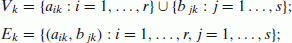
Comment: vertex a ik represents F i at period k, for i = 1, ..., r, k = 1, ..., t; vertex b ik represents O j at the period k, for j = 1, ..., s, k = 1, ..., t; edge (a ik , b jk ) represents the possibility of transporting good from F i to O j at period k, for i = 1, ..., r, j = 1, ..., s, k = 1, ..., t.
-
add vertex σ and edges {(σ, a ik ) : i = 1, ..., r, k = 1, ..., t};
-
add vertex τ and edges {(b jk , τ) : j = 1, ..., s, k = 1, ..., t};
-
add edges {(a ik , aik + 1) : i = 1, ..., r, k = 1, ..., t − 1};
-
add edges {(b jk , bjk + 1) : j = 1, ..., s, k = 1, ..., t − 1};
-
the elements of V and E are defined as above;
-
the function
 of edge-capacities is defined as follows:
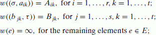
-
the function
 of edge-costs is defined as follows:
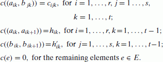


 of edge-capacities is defined as follows:
 of edge-costs is defined as follows:
Let N = (σ, τ, V, E, w, c) be the network defined as above. By Eq. 1 it is possible to define in N a flow of value v f = ∑ j = 1,...,r ∑ k = 1,...,tB ik . Then let P f denote the min-cost flow problem in (N, v f ).

A min-cost flow model for P in the case r = 2, s = 2, t = 3
By Eq. 1 and by the structure of N, given a feasible solution [x ijk , z ik , z′ jk ] of P one can derive a feasible solution [y(u, v)] of P f , and vice-versa, by the following equalities:
-
x ijk = y(a ik , b jk ) for i = 1, ..., r, j = 1, ..., s, k = 1, ..., t;
-
z ik = y(a ik , aik + 1) for i = 1, ..., r, k = 1, ..., t;
-
z′ jk = y(b jk , bjk + 1) for j = 1, ..., s, k = 1, ..., t.
Furthermore C[x ijk , z ik , z′ jk ] = ∑ (u,v) ∈ Ec(u, v)y(u, v), by the definition of costs for edges of N.
One can formalize what above by the following theorem.
Theorem 1
An instance of P can be solved as a min-cost flow problem.
As network N can be efficiently constructed, one obtains the following corollary.
Corollary 1
Problem P can be solved in polynomial time.
In particular the problem admits an optimal integer solution if all the values A ik , B jk are integer.
3 A Hitchcock model for P
Let us consider problem P as problem P f defined in Section 2, according to the equalities linking the respective solutions. In [10] a standard transformation from an instance of the min-cost flow problem to an instance of the Hitchcock problem is shown. However, in the sequel let us try to model P as a Hitchcock problem just by exploiting some peculiarities of the problem (i.e., by compacting some aspects of P f ) and not by using the standard transformation of [10].
The Hitchcock model for P is based on the following variables (see Fig. 2):

Then (also by conditions (1) and (2)) one has:


It remains to define the costs cii′jj′.

A Hitchcock model for P in the case r = 2, s = 2, t = 3 (the edges, i.e. the variables, with i′ > j′ are omitted)
Assume that i′ > j′. Then one can define cii′jj′ = ∞, so to ensure qii′jj′ = 0 for i′ > j′.
Assume that i′ ≤ j′.
Let us observe that for any solution of P, the amount qii′jj′ will arrive from F i to O j through a path from aii′ to bjj′ in the network N of Section 2: in particular, all the edge-capacities along each of such paths are ∞.
It follows that for any optimal solution of P, the amount qii′jj′ will arrive from F i to O j through a least cost path (or in general through least cost paths, if more than one) from aii′ to bjj′ in the network N of Section 2. Then the cost cii′jj′ may be defined as the cost of a least cost path from aii′ to bjj′: by the structure of N such paths are exactly j′ − i′ + 1 (i.e., each such path is formed by a possible storage multi period in F i , by a transfer period from F i to O j , and by a possible storage multi period in O j : the transfer period is a period k with i′ ≤ k ≤ j′).
Then summarizing one obtains:
-
cii′jj′ = ∞, for i′ > j′;
-
cii′jj′ = mini′ ≤ k ≤ j′ {( ∑ u = i′,...,k − 1h iu ) + c ijk + ( ∑ u = k,...,j′h ju )}, for i′ ≤ j′.
Then the objective function ∑ i = 1,...,r ∑ i′ = 1,...,t ∑ j = 1,...,s ∑ j′ = 1,...,tcii′jj′qii′jj′ and the constraints (3), (4), (5) define an instance of the Hitchcock problem (all the costs are non-negative), say H.
Let us show that given an optimal solution [x ijk , z ik , z′ jk ] of P one can derive a feasible solution [qii′jj′] of H, and vice-versa.
From P to H Let [x ijk , z ik , z′ jk ] be an optimal solution of P. Then a solution [qii′jj′] of H with the same cost can be obtained as follows. Let us observe that: (i) the costs of storage in facilities (in outlet) do not depend on the destination (on the origin) of the good. By (i) and by the definition of costs cii′jj′, one may proceed as follows.
The first step may be to obtain the values of q ikjk , for k = 1, ..., t: to this end, for k = 1, ..., t, it is enough to chose the values of q ikjk , in order to maximize ∑ i = 1,...,r ∑ j = 1,...,sq ikjk , subject to q ikjk ≤ x ijk and to ∑ j = 1,...,sq ikjk ≤ A ik for i = 1, ..., r (that is to charge the values of x ijk to those of q ikjk as much as possible). That can be easily done by a greedy technique.
The second step may be to obtain the other values of qii′jj′: to this end one can apply the Ford–Fulkerson procedure to compute a maximum flow in the network N′ obtained from the network N of Section 2 by modifying the edge-capacities as follows:
-
w((σ, a ik )) = A ik − ∑ j = 1,...,sq ikjk , for i = 1, ..., r, k = 1, ..., t;
-
w((b jk , τ)) = B jk − ∑ i = 1,...,rq ikjk , for j = 1, ..., s, k = 1, ..., t;
-
w((a ik ,aik + 1)) = z ik , for i = 1, ..., r, k = 1, ..., t;
-
w((b ik , bik + 1)) = z′ jk , for j = 1, ..., s, k = 1, ..., t;
-
w((a ik , b ik )) = x ijk − q ikjk , for i = 1, ..., r, j = 1, ..., s, k = 1, ..., t.
In fact, by starting from a null flow in N′, at each iteration of the procedure an augmenting flow saturates a path in N′ from a certain lowest aii′ to a certain highest bjj′, with i′ < j′ (because of the first step): the value of such an augmenting flow can be charged onto qii′jj′, which may be updated at each iteration. Note that: concerning the cost, [qii′jj′] has the same cost as [x ijk , z ik , z′ jk ], since the latter is an optimal solution of P and by the definition of costs cii′jj′; concerning the procedure, at most t × (r × t) × (s × t) iterations occur, where the first t stands for an upper bound to the number of all possible paths from aii′ to bjj′.
From H to P Let [qii′jj′] be a solution of H. Then a solution [x ijk , z ik , z′ jk ] of P with the same cost can be obtained as follows. By the definition of costs cii′jj′, every qii′jj′ defines a least cost path Pii′jj′ from aii′ to bjj′ in the network N of Section 2 (i.e., corresponding to the costs which minimize the expression which defines cii′jj′). Then qii′jj′ can be charged (as a flow line) onto the edges of Pii′jj′, so to compose the values of a solution [x ijk , z ik , z′ jk ] of P according to the equalities of Section 2.
One can formalize what above by the following theorem.
Theorem 2
An instance of P can be solved (directly) as a Hitchcock problem.
Then a corollary and a comment similar to those at the end of Section 2 hold.
4 Some generalizations of P
In this section let us introduce three possible generalizations of problem P, pointing out the advantages and the disadvantage of the two proposed models.
Let P1 be the following problem. In the context of problem P, assume that every facility F i for i = 1, ..., r (that every outlet O j for j = 1, ..., s) can store at most d i (at most d′ j ) units of good at the end of each period k for k = 1, ..., t. The objective remains that of the problem P.
Then P1 can be modeled by the min-cost flow model of Section 2, by modifying the network N as follows:
-
w((a ik , aik + 1)) = d i , for i = 1, ..., r, k = 1, ..., t;
-
w((b jk , bjk + 1)) = d′ j , for j = 1, ..., s, k = 1, ..., t.
Then P1 can be solved as a min-cost flow problem, i.e., in polynomial time.
On the other hand, it seems to be not immediate to model P1 by the Hitchcock model of Section 3.
Let P2 be the following problem. In the context of problem P, assume that the good produced in a facility has to be sold in a outlet before a certain number of periods (e.g., before corruption of the good), say L periods. The objective remains that of the problem P.
Then P2 can be modeled by the min-cost flow model of Section 2, by adding the following constraints:
-
 , for k = 1, ..., t, where k* = min{k + L, s}.
 , for k = 1, ..., t, where k* = min{k + L, s}.
Actually in this way one obtains a generalization of the min-cost flow problem, which remains a linear programming problem, but can not be solved as a classical min-cost flow problem.
Then P2 can be modeled by the Hitchcock model of Section 3, by modifying the costs as follows:
-
cii′jj′ = ∞ , for j′ − i′ > L,
so to ensure qii′jj′ = 0 for j′ − i′ > L.
Then P2 can be solved as a Hitchcock problem, i.e., in polynomial time.
Let P3 be the following problem: In the context of problem P, let c ik (i = 1, ..., r, k = 1, ..., t) be the cost of production for a unit of good in F i in the k-th period, and let p jk (j = 1, ..., s, k = 1, ..., t) be the profit for selling a unit of good in O j in the k-th period: in particular, A ik can be view as the maximum amount which can be produced by F i in the k-th period. Then one wishes to minimize the total cost of transportation, of storage, and of production, less the total profit by selling, along the horizon of t periods, i.e., one wishes to maximize the total profit by selling, less the total cost of transportation, of storage, and of production, along the horizon of t periods.
A possible scenario for problem P3 may be that of a tobacco manufacture company: in fact the selling price of tobacco varies over countries and its fluctuation (over countries) is planned in advance.
Then P3 can be modeled by the min-cost flow model of Section 2, by modifying the network N as follows:
-
c((σ, a ik )) = c ik , for i = 1, ..., r, k = 1, ..., t;
-
c((σ, b jk )) = − p jk , for j = 1, ..., s, k = 1, ..., t.
Actually in this way one obtains a generalization of the min-cost flow problem (where: the costs are allowed to be negative, and the flow value is not fixed), which remains a linear programming problem, but can not be solved as a classical min-cost flow problem.
Then P3 can be modeled by the Hitchcock model of Section 3 as follows.
Let us observe that (recalling the definition of costs cii′jj′ of Section 3) it is possible and convenient to send good from aii′ to bjj′ if and only if:
-
i′ ≤ j′ (it is possible);
-
cii′ +mini′ ≤ k ≤ j′ {( ∑ u = i′,...,k − 1h iu ) + c ijk + ( ∑ u = k,...,j′h ju )} − pjj′ < 0 (it is convenient).
Let us say that a variable qii′jj′ is green if the above two conditions are satisfied.
For any green variable qii′jj′ let us write  cii′ + mini′ ≤ k ≤ j′ {( ∑ u = i′,...,k − 1h
iu
) + c
ijk
+ ( ∑ u = k,...,j′h
ju
)} − pjj′, and let K be a scalar with
cii′ + mini′ ≤ k ≤ j′ {( ∑ u = i′,...,k − 1h
iu
) + c
ijk
+ ( ∑ u = k,...,j′h
ju
)} − pjj′, and let K be a scalar with  .
.
Then let us define the following costs  for every variable qii′jj′:
-
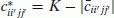 , if qii′jj′ is a green variable;
 -
 , otherwise.
 , if qii′jj′ is a green variable;
 , otherwise.
Let  denote the Hitchcock problem (with all nonnegative costs) defined by the objective function
  and subject to the constraints of the Hitchcock model of P.
Then it is not difficult to verify that, given an optimal solution [ ] of
] of  , one can directly derive an optimal solution [qii′jj′] of P3 by setting:
-
 , if qii′jj′ is a green variable;
 -
qii′jj′ = 0, otherwise.
 , if qii′jj′ is a green variable;
Then P3 can be solved as a Hitchcock problem, i.e., in polynomial time.
Then summarizing it seems that: the first model is more powerful than the second model to describe generalizations of P (e.g., P1), though it may lead to linear programming which can not be solved as a classical min-cost flow problem (e.g., P2 and P3); while the second model may be more useful than the first model to show that certain generalizations of P (e.g., P2 and P3) can be solved as a classical Hitchcock problem.
5 Conclusions
The (Hitchcock-) transportation problem is a well known problem in operations research [6, 9, 10] and can be solved in polynomial time by fast algorithms (see e.g. [12]). By its applicative nature, several versions of this problem have been considered, such as dynamic, time-dependent versions (see e.g. [5]).
In particular the following time dependent version was studied in [2] (see also [3, 4]) by referring to a method for solving integer programming which resorts to the calculation of suitable Gröbner bases [7]:
Given r production facilities F1, ..., F r , let A ik (i = 1, ..., r, and k = 1, ..., t) denote the number of units of an indivisible good produced by F i during the k-th period of a planning horizon of t periods. Assume that there are s outlets O1, ..., O s each one demanding a certain number of units per period, say B jk (j = 1, ..., s and k : = 1, ..., t). Let c ijk ≥ 0 be the cost associated with transporting one unit from F i to O j during the k-th period, let h ik ≥ 0 (let h′ jk ≥ 0) be the cost associated with storing one unit in F i (in O j ) at the end of the k-th period. Then one wishes to minimize the total cost of transportation and of storage along the planning horizon of t periods.
In this paper we tried to study the above problem by an operations research approach. We described the problem by two models, showing that it can be solved in polynomial time by standard software packages: the first is a natural min-cost flow model, while the second is a Hitchcock model obtained by exploiting some peculiarities of the problem. Then we described some possible generalizations of the problem by adapting the two proposed models, pointing out that each model seems to provide different benefits.
References
Bein W, Brucker P, Park JK, Pathak PK (1995) A Monge property for the d-dimensional transportation problem. Discrete Appl Math 58:97–109
Boffi G, Rossi F (2000) Gröbner bases related to 3-dimensional transportation problems. In: Quaderni matematici dell’ Universitá di Trieste, vol 482. DSM-Trieste. http://www.dmi.units.it/~rossif/
Boffi G, Rossi F (2001) Lexicographic Gröbner bases of 3-dimensional transportation problems. In: Symbolic computation: solving equations in algebra, geometry, and engineering (South Hadley, MA, 2000). Contemporary Mathematics, vol 286. Amer. Math. Soc., Providence, pp 145–168
Boffi G, Rossi F (2006) Lexicographic Gröbner bases for transportation problems of format r ×3 ×3. J Symb Comput 41:336–356
Bookbinder JH, Sethi SP (1980) The dynamic transportation problem: a survey. Nav Res Logist Q 27:65–87
Cook WJ, Cunningham WH, Pulleyblank WR, Schrijver A (1998) Combinatorial optimization. Wiley, New York
Hosten S, Thomas R (1998) Gröbner bases and integer programming. In: Bichberger, Winkler (eds) Gröbner bases and applications, vol 251. Cambridge University Press, Cambridge, pp 144–158
Klein RS, Luss H, Rothblum UG (1995) Multiperiod allocation of substitutable resourses. Eur J Oper Res 85:488–503
Lawler E (2001) Combinatorial optimization: networks and matroids. Dover, New York
Papadimitriou CH, Steiglitz K (1998) Combinatorial optimization: algorithms and complexity. Dover, New York
Sturmfels B (1995) Gröbner bases and convex polytopes. AMS, Providence
Tokuyama T, Nakano J (1995) Efficient algorithms for the Hitchcock transportation problem. SIAM J Comput 24:563–578
Acknowledgements
I would like to thank Prof. Giandomenico Boffi and Prof. Fabio Rossi for having kindly explained their work [2] in 2003. Then would like to thank the referees for their comments. Finally would like humbly to dedicate this paper to (the memory of) my grandfather Raffaele Mosca.
Author information
Authors and Affiliations
Corresponding author
Rights and permissions
Open Access This article is distributed under the terms of the Creative Commons Attribution 2.0 International License (https://creativecommons.org/licenses/by/2.0), which permits unrestricted use, distribution, and reproduction in any medium, provided the original work is properly cited.
About this article
Cite this article
Mosca, R. A time expanded version of the (Hitchcock-) transportation problem. Eur. Transp. Res. Rev. 3, 161–166 (2011). https://doi.org/10.1007/s12544-011-0056-3
Received:
Accepted:
Published:
Issue Date:
DOI: https://doi.org/10.1007/s12544-011-0056-3