Assessing robustness in multimodal transportation systems: a case study in Lisbon

Abstract

Introduction

Worldwide public transport systems are exposed to disruptions caused by malfunctions, accidents, maintenance, reduced fleet, and disasters, compromising mobility. Transport networks’ multimodal planning and management can be explored to increase their robustness against these events. In this context, this research paper proposes and empirically compares methods to assess the robustness of a multimodal transport network, looking at aspects regarding the single-mode and multimodal network topology.

Materials and Methods

We hypothesize that the appropriate multilayered and traffic sensitive modeling of a multimodal transport network can help characterize robustness and further unravel vulnerabilities related to the integration of different transport modes. Using metric-based targeting, we evaluate how the network decreases performance when simulating failures on stations and pathways using different scenarios. The following six extraction strategies for nodes and edges were used in the simulation: Random removal; Initial Degree removal; Initial Betweenness removal; Recalculate Degree removal; Recalculate Betweenness removal; and Multimodal Hubs removal. Lisbon’s public transport is used as a case study and is modeled as a multiplex network integrating eight different modes of transport. Proposing a novel normalized version of assessing the impact of failures, we were able to compare side by side the robustness of each modality layer, regardless of their size. Lastly, we simulate cascading events such as the breakdown of an entire transportation line.

Conclusions

Using different ways to induce failures in the network, we observe that to leave all nodes completely disconnected, we would need to remove about half the network nodes, highlighting the robustness of the Lisbon public transport network. Comparing different failure scenarios, methods that rely on recalculating network metrics yield a higher impact on the network robustness assessment. The impact of different events is quantified, showing that failures in stations are generally more dangerous than in pathways and offering views on the consequences of deactivating particular network modules. Overall, the results of this study allow decision-makers to gain further understanding of the topological vulnerabilities of a transportation network.

1 Introduction

Around 55% of the world's population lives in urban areas [37]. However, such areas represent only a minor percentage of the total surface area. Therefore, daily commuting patterns and mobility services’ consumption impact factors such as the usage of natural resources and impact time in transportation, pollution, and quality of life, among others, yield extreme importance in sustainable development goals [3, 4, 6]). In this context, numerous studies attempt to optimize transportation systems planning and usage in urban scenarios [10, 28, 30].

Among the studied solutions, the importance of a multimodal transportation system arises due to the high demand for some traffic corridors. According to [21], an improved articulation of multimodality aspects within a transport system is significantly associated with lower carbon emissions. This assertion leads us to believe that successfully coordinating the interfaces in this kind of network is a viable solution for promoting carbon neutrality in the long run. However, according to [15], the study of multimodal transportation systems “has historically been underrepresented in travel surveying efforts. This lack of consideration has implications for widely accepted statistics for nonmotorized travel behavior (walking, bicycling, among others). It affects researchers and professionals in travel modeling, urban planning, public health, and urban design”. An integrated view of how specific failures affect the overall multimodal system is also relevant. Since it is relatively common to have planned or unplanned disruptions (i.e., construction works, technical failures, attacks, and natural disasters), causing delays and possibly inhibiting the usage of a pathway or station [11]. This observation raises the need to assess how robust these transportation systems are. Therefore, our main research objective is to assess the robustness of multimodal transportation systems in an urban scenario. In the context of this study, this assessment is applied at a topological level. Particularly we would like to understand how the different types of percolation tests have different results depending on network topology, the main topological fragilities regrading mono and multimodal public transport, and the differences between them and a metric to access the topological robustness of the network, that allows for direct comparison regardless of the network size and shape.

Making stops along our path from origin to our destination is often required, and the more stops we make, the more time we spend on transportation. So naturally, how nodes and edges failures affect the Average Path Length (APL) is an important research question that we are interested in answering. This is the case since the effectiveness of a path between two stations can be assessed by the number of stops in a trip (the APL). Besides the effects on the APL, understanding how many nodes (or stations) have to fail to fragment the network into isolated components is a requirement to understand further the impact of a disaster on a station or stop (in creating isolated components). In addition, we also aim to infer the effect of removing edges (pathways) versus nodes (stations) since this helps us infer if incidents have a higher impact on pathways or stations. To empirically test the simulation-based robustness testing, we aim to understand if metrics should be recalculated after each extraction and the measurement of the impact of cascading failures. Such as what happens if a station failure causes chain reactions on other stations located along the same line or in the nearby stations or stops from other modes.

The current study contributes to increasing the knowledge of the robustness assessment of multimodal transportation systems. Hence, we do a comprehensive review of modeling multimodal transportation systems and quantitatively assess their robustness. Another contribution of this study is the possibility of supporting public transportation policies focusing on actionable priorities for a more resilient system design. For instance, where should the focus of actionability be in case of an accident on different stations or pathways. By understanding which elements are more important for network integration.

For this research, the city of Lisbon is used as an example to improve the integration of the current multimodal transport network. This analysis is fundamental in the context of the Lisbon Metropolitan Area (LMA), where the average occupancy rate for individual private transport (cars) is 1.60 passengers per vehicle. This is also where the daily traffic inflow in the county of Lisbon is also the cumulative result of commuting traffic inflows between Lisbon and the eighteen municipalities that integrate the LMA [24]. Several road traffic corridors are flooded daily with single occupancy vehicles that could use another public transport alternative. Despite stable establishments and integrating the operators’ systems with a single card, challenges to the public transport network's integrated operation and multimodal planning still persist within LMA.

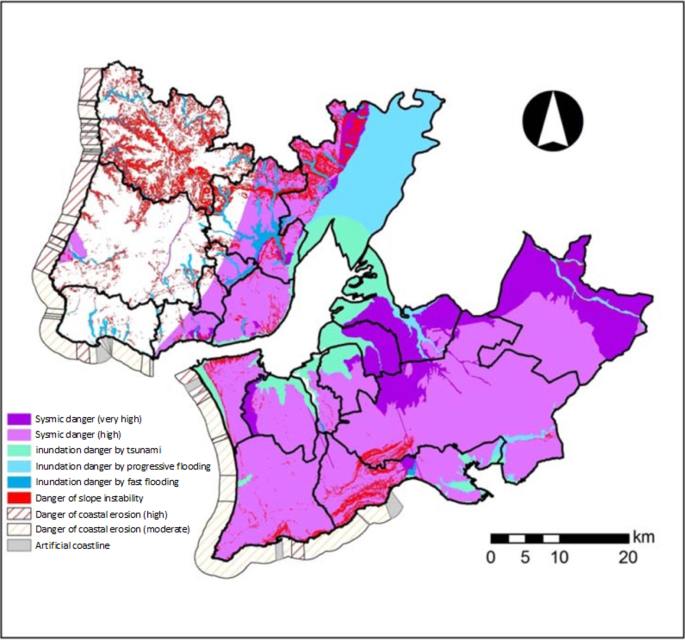
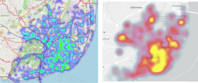
Additionally, as noted previously, in a general sense, it is essential to note the impact of natural hazards on disrupting a working transportation system as well. Previous literature [32] denotes the natural hazard risk in different zones of the LMA (see Fig. 1). This map shows us the spatial distribution of risk for earthquakes, flooding, and landslides in the county of Lisbon. This stresses the importance of understanding various risk impacts on the network's structure. Along with the general risk from natural incidents, other incidents through the city have a higher incidence rate, and these usually have a more localized effect [19]. Such incidents may be caused by faults in energy and water suppliers, traffic accidents, and fires that disable stations and pathways. [19] rendered a map of incidents from a diverse standpoint (see Fig. 2). This shows us that a study on the impact of network robustness at a local level is relevant.

Fig. 1

Lisbon Metropolitan Area, natural hazard map, extracted and translated from [32]

Fig. 2

Distribution of incidents in the city of Lisbon from [19]. On the right is the occurrence of incidents and on the left, their impact on pathways, i.e., the number of roads affected

Since the Lisbon public transportation network is susceptible to these failures that can affect the daily commute of its users, a way to guarantee and improve the robustness of this critical component of our public services is crucial. To tackle this problem, we aim to understand how robust the Lisbon public transport network is. This assessment starts by quantitatively measuring robustness [40]. Since the Lisbon public transportation network is also complex, examining how different stations and stops may have similar properties, bridging different lines (routes as linear road/rail/other mode infrastructures) and transportation modes is essential. Topological attributes and concepts of network resilience, besides simulation, will play a role in this research study. We ask ourselves which nodes (e.g., stations) are central and the role of degree-degree correlations. This is, if central stations connect to other central stations in this particular topology, this may cause a higher fragility [41]. Also, looking at how different extraction strategies (or simulations) for quantifying robustness affect the connectedness of the network will shed some light on which method has the highest impact on breaking the critical pathways that keep the transportation system usable throughout the city.

The above concepts will be applied to Lisbon’s multimodal transport network in the ILU (Integrative Learning from Urban data and the situational context for city mobility optimization) project. This project joins research institutes, the Lisbon municipality, and public transportation operators to promote more efficient and sustainable mobility.

2 Literature review

Robustness can be understood as the quality of the capability of a system to work under disruptions [23]. Robustness has been alternatively defined as an optimization problem [26]. A robust solution can be seen as having the best performance under high-stress conditions. To further understand this property of the system perturbation, the literature review shows that experiments are a dominant approach, which can be done in silico (using computer simulations) [29]. In the context of a multimodal transportation system, we can inherently see the redundancy since the transportation modes usually provide alternative routes for the same places.

Previous studies indicate that the first step in measuring the robustness of a transportation system is to model the transportation network. Accordingly, the modeling of multimodal transportation systems recurring to multilayer networks has been previously proposed to analyze urban transportation systems [2]. This allowed the analysis of superlayer interdependence. Multilayer networks are also used to model air transportation networks. This can, for instance, be used to study how the degree–degree correlations of a network affect the spreading of an epidemic [5]. Different types of multimodal transport networks have been modeled in several empirical studies, as shown in Table 1 [39]. Note that air travel can be modeled as a heterogeneous mode of transport, as different air travel companies constitute different layers of a network [20].

Table 1 Empirical studies of multilayer transportation networks by Zhan et al.

Different authors have modeled and assessed diverse types of networks. [8] addressed the evolution along time using historical data. [36] developed a method for choosing different routes in shipment according to demand. [16] studied connectedness in India using community membership and betweenness centrality. [38] applied a weighted multiplex to air traffic to then make a network analysis with metrics such as average degree and assortativity.

[18] modeled an air traffic network in layers based on flight frequency and concluded that it is less redundant in the Chinese network than the worldwide network. [5] modeled an air traffic network and assessed assortativity and rich-club effect (nodes with high degrees connect to nodes with high degrees) in international flights. [2] modeled the Madrid urban transport network, the measured overlap between different modes and transfers, and the time from one station to another. [17] studied how the network's topology affected the formation of communities and how betweenness centrality and closeness centrality affect growth. [27] create a methodology to assess the spatial accessibility of public transportation networks using a case study in Shanghai, China.

To answer the need for measuring the resilience of networks, [25] noted in their robustness and resilience review that a network should be considered resilient if it sustains a high number of node failures before it becomes disconnected. In that sense, performing node percolation tests is suggested to measure resilience. Measuring this property in transport networks has been the focus of several studies. [35] have evaluated system-wide robustness by finding critical isolating links in road networks. They reduced the link capacity and measured the travel time to measure robustness. This allowed for a dynamic perspective as well. Later on, [42] conducted a similar study but induced the vulnerabilities by blocking lanes instead, same as deleting an edge, which ranked the links by how critical they were building upon the much earlier work that did just that [33].

These studies are related to the earlier studies on reliability by [13], where they measured the reliability of networks given the demand change based on route choice models. This study extended capacity reliability to network equilibrium models as well as accounts for route-choice actions of drivers. [1] measured the reliability using network capacity and travel time by changing demand and inducing link degradation and non-persistent congestion. These studies show how different demand levels affect capacity and reliability in an analytical way. It is important to note that reliability is fundamentally different from resilience. Reliability is usually a measure of susceptibility to the interruption of service. Resilience, on the other hand, measures the ability to recover from such interruptions in service [14]. Robustness, on the other hand, can be seen as a dimension of resilience and as a cause for reliability.

Studies of network resilience have also been done in the context of multimodal transport. [31] recently showed that the same idea of percolation could be used in multiplex networks. This notion opens this test as a way to measure the robustness of multimodal transport networks accurately.

Another view on resilience measurement on multimodal transport networks is given by [7], who postulates that a whirlpool network structure on a multimodal transport network leads to a cyclic steady state, unlike a tree structure, under the flow simulations proposed. A whirlpool state is one that points towards another, and the following states recursively point to the following until it completes a circle. Then the measurement of robustness is given by the ratio of states in a whirlpool structure and the total number of states in the multimodal transport network.

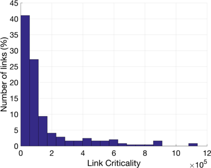
Besides a topological resilience test, dynamic measurement of such property has also been studied in multimodal urban transport. [34] studied resilience to extreme weather events (EWE) in several European cities by measuring the percentage of change in working segments during the EWE. Then claimed this could be used for prediction tasks by using past rail, air, and road usage data. However, this method lacked actionable information because prevention is only attainable if we know where to act. Later on, [12] defined a framework to assess robustness. This helped the description of robustness assessment as an economic problem. This kind of assessment is very relevant for this study because it provides a baseline for understanding the impact of different disruption scenarios in specific links, quantifying their criticality. This is a type of assessment that provides specific enough data to be actionable in the real world, showing that the number of critical links distribution follows a left-skewed behavior (Fig. 3). This is relevant since we can see that most links are not that critical, and others are significant to keep the network connected. By identifying such links and providing redundancy, priority policies, and other measures, the robustness of the network can actually increase.

Fig. 3

[12] link criticality study results

3 Methods and modelling

3.1 Methods

To answer the questions stated in the introduction regarding the topological robustness, we use different strategies. As we have seen, there are several approaches to assessing robustness. One of them is removing nodes or edges from a network to measure the impact of a simulated station failure [31]. The simplest way to do this is by injecting random failures in the network, i.e., randomly removing nodes from the network. It is expected that this simple strategy may not maximize the damage to the network, but it can be a reasonably realistic approach since the Lisbon public transport network may have station failures due to unpredictable and unexpected events.

Other more precise strategies were defined by [22], and we followed their strategy. We also simulated the failure of nodes and edges to be able to compare, which yields the highest impact, as the optimization stress handling can be part of the definition of robustness, as seen previously. These more precise node extractions (simulated station failures) utilize attributes from the network, such as degree and centrality. To test a network with more precision, an effective strategy should be to extract the most critical node. This notion of importance can vary depending on the attribute to which we give attention.

We could select nodes in descending order of degree. This extraction is called Initial Degree removal—ID removal—because we base the extraction on only the initial calculation of the degrees, and we do not update it after removing nodes.

Another critical attribute is the centrality of a node. There are a few types of centralities, but the betweenness centrality is crucial since it represents the nodes that have edges that unify communities/groups inside the network. These nodes are the ones with the highest criticality for network connectivity since they connect the communities of the network. This extraction is called Initial Betweenness removal—IB removal—like ID removal, it only calculates the initial betweenness centrality of each node at the beginning and does not update it.

Both extractions only calculate the attributes, degree distribution, and betweenness centrality at the beginning of the algorithm. When we remove nodes from the network, it changes the degree of the neighbors of the removed node, and it modifies the betweenness centrality of all the nodes. Two new strategies appear called Recalculate Degree removal—RD removal—and Recalculate Betweenness removal—RB removal. These strategies are identical to the ID and IB ones, except they update/recalculate the degree and the betweenness centrality after each node/edge removal. The RD and RB algorithms are considerably more time and computation expensive for each interaction, but we wanted to study if they are more efficient at disconnecting the network. Efficiency, in this case, is a way to simulate the highest stress levels.

ID and RD removal are local strategies because when a node is removed, it only changes the degree of the neighbors of that node. Thus, only these local nodes need to be updated. On the other hand, IB and RB removal are global strategies since by removing a node, we need to recalculate the betweenness centrality globally, i.e., of all nodes.

Every calculation of the betweenness centrality of the network costs around 5 min, and since we must apply thousands of recalculations (one per node removal), this would be very time-consuming and less sustainable. Because of that, we decided only to recalculate the betweenness centrality when batches of 5% of the nodes were removed. Being N the number of Nodes and E the number of Edges, the ID algorithm is ${\text{O}}\left( {{\text{N}} + {\text{E}}} \right)$, the RD is ${\text{O}}\left( {{\text{N}}\left( {{\text{N}} + {\text{E}}} \right)} \right)$, and the IB is ${\text{O}}\left( {{\text{NE}}} \right){ }$(using a faster algorithm for betweenness centrality created by [9]), and the RB is ${\text{O}}\left( {N^{2} {\text{E}}} \right)$.

3.2 Modeling

Most worldwide public transportation networks are multimodal. Therefore, these are modeled as multilayers. Moreover, we also wanted to test if removing nodes that connect layers of the graph is critical, i.e., if it disconnects the network faster. We call these nodes multimodal hubs, and this extraction strategy is Multimodal Hubs removal. For example, two multimodal hubs are Alameda, which connects Metro and Carris, and Gare do Oriente, which connects Carris, Metro, and CP. It is worth noting that the Multimodal Hubs removal strategy only makes sense when evaluating the multilayer network. When evaluating each modality, this strategy is invalid because there are no multimodal hubs.

Removing nodes from this network may correspond to a stop being deactivated or being in construction, while removing edges may correspond to cutting roads or accidents preventing any vehicle from passing through. Edges can also fail. All our node extraction strategies can be applied to edges with a few modifications. For example, how can we get the degree of an edge? The edge degree depends on the nodes that are connected by it. We used the following four different methods to calculate edge degrees:

• A. $k_{e} = k_{v} \cdot k_{w}$

• B. $k_{e} = k_{v} + k_{w}$

• C. $k_{e} = {\text{min}}(k_{v} , k_{w} )$

• D. $k_{e} = {\text{max}}(k_{v} , k_{w} )$

where ke is the edge degree and kv and kw are the degree of the nodes that are connected by the edge e. Since our network is directed, we also assume that v is the source and w is the destination node of the edge. However, there are other ways to calculate the degree of an edge, such as ke = kv or ke = kw.

In accordance with the study of [22], where they concluded that method A. ke = kv ∗ kw was the best fit for the majority of the network types that they studied. Method A showed the best correlation of the four methods between the edge degree and the edge betweenness centrality. It is expected that the node with a higher degree should also have a higher betweenness centrality. To calculate the betweenness centrality of an edge, we also used the [9] ${\text{O}}\left( {\text{ NE}} \right)$ algorithm.

We can expect that the extractions based on centrality measures may be more harmful than the random failures. Concerning the nodes vs. edges, we believe that there could be a slight difference between these extractions, but this is hard to predict. Degree-based strategies probably will split the network into many subgraphs of vertices with low degrees. Betweenness centrality strategies can create clusters that are highly connected since they tend to destroy the bridges that connect communities first.

We understand that not only single nodes fail but also more catastrophic events can happen in the network, bringing the notion of cascading effect. For the cascading effects, we described and implemented two extraction strategies.

The cascading effect simulating a Line Failure removes an entire transportation line in the network. This could happen with an underground implosion that made the whole line stop. We simulate this by removing all the nodes that have the attribute of that line. Some nodes may belong to more than one line, even from different modalities. For example, Gare do Oriente stop is a multimodal hub that belongs to Metro, Carris, and CP (railway company).

The cascading effect simulating a Neighbours Failure removes neighbors from several layers of a failed node. One example of this in the Lisbon public transportation network could be a recursive failing of transports in the same spot. When a station fails, the neighbor stations could experience overflows because of relocated traffic, and this could potentially cause them to fail as well. To simulate this type of cascading effect, we collect several layers of the node’s neighbors, and then remove all these nodes at the same time. An example of this could be a flood that affected all transport modes in a particular spot of the city to the point of not being usable. In conclusion, we used the six following extraction strategies for nodes and edges:

• (1) Random removal

• (2) Initial Degree removal (ID)

• (3) Initial Betweenness removal (IB)

• (4) Recalculate Degree removal (RD)

• (5) Recalculate Betweenness removal (RB)

• (6) Multimodal Hubs removal

We also used the two following extraction strategies for cascading effects:

• (1) Line Failure

• (2) Neighbours’ Failure

3.3 Assessment metrics

To assess the impact of each strategy, we explore the impact of each removal based on different metrics through the simulations. To understand how connectedness is affected, we measure the average path length (also known as average geodesic distance), average degree, number of isolated components, and the size of the strongly connected component [5, 16, 38]. To understand how the average path length is impacted by each removal, we only average out the shortest paths that still exist in the network. This approach allows us not to need to calculate the inverse path length, $l^{ - 1}$. As the study of this network is applied to a multimodal transportation network, we also measure the impact of the described extractions on the use of multimodality.

By implementing the different extraction strategies discussed previously. For each iteration, we compute the largest SCC and its size. This size decreases with the removal, and if a critical station is removed, the size decreases even faster. Ergo the strategy which has a faster decrease has a more significant impact on the network. This means that networks that exhibit a steeper decrease sooner, as the percentage of iteration steps, are less robust. In the same fashion, a high-performance extraction strategy is one in which the SCC descends faster.

To compare different removal strategies, we propose a novel metric, the discrete normalized Area Under Curve (AUC), to compare the resilience of the different layers and the multilayer network. The normalized AUC ⊂ [0,100] allows us to compare the values of networks of different sizes and shapes. This is calculated using the following formula:

$$AUC_{Normalized} = \sum\limits_{i = 0}^{{\upchi }} {\frac{{{\uptau }_{i} }}{V}} \cdot \frac{100}{{\upchi }}$$

where ${\upchi }$ is the number of steps of the simulation, ${\uptau }_{i}$, is the size of the largest strongly connected component at timestep $i$, and $V$ is the number of nodes of the network. This measurement allows us to compare the different resilience side by side. It is important to note that this metric might have a higher variability (for both inflation and deflation) in smaller networks, given the granularity.

4 Results and discussion

4.1 Data extraction and pre-processing

Firstly, we identified the criteria used for the inference of the multiplex network, followed by an analysis of the robustness of the topology. To transform route planning from GTFS data files of each mode into a network, we joined the routes and the stops of each one of the transportation modalities: Carris, CP, Fertagus, Metro, Rodlisboa, Sulfertagus, Transtejo, and TST (bus, railway, riverway, subway, tram companies’). This merge contains information regarding the id, geographical position, sequence within the line, and name of the station. This allows us to verify which stops are connected to one another.

Given the structure of the data, we created a directed graph (digraph) for each transportation modality (bus, railway, riverway, subway, tram), forming a layer for each. We resorted to digraphs for each layer because transport does not always flow in both directions within the same path. This allows us to create each layer of our multilayer network. We apply a multilayer representation hence the edges of different layers have different types that represent different realities. Modeling such characteristics is not possible with a single layer (or monolayer) network.

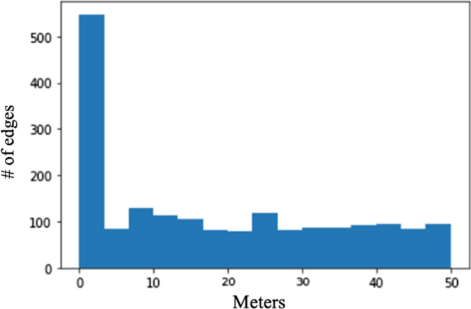
After the representation of each layer, we must account for possible multimodal interactions, i.e., the possibility to shift to different transportation modes within a trip. These links are of extreme importance because they allow us to assess the connectivity of the transportation system as a whole. To accurately understand where these edges could be located, we created a script that extracted the Lisbon city map and calculated the walking distance between every two stations, and combined it with a standard coordinate distance calculation to get faster calculations (Fig. 4). After getting this result, we selected the pairs of stations from different modes and linked them based on distance. The intermodal interfaces are about 0,0040% of the distances calculated. We connected the eight modes of transportation in the city of Lisbon using the described method.

Fig. 4

The distribution of distances associated with the 1878 intermodal connections has a very high cardinality of distances close to 0 m. This represents the stations/stops that simultaneously link layers

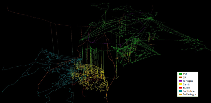
By programming a 3-dimensional method for visualizing such a network, using the geographical information available, we were able to see its structure (Fig. 5). This network is composed of 8 layers, 7972 nodes, and 11,892 edges. The complete network required the computation of 46 399 492 distances to join all the layers with the multimodal connections.

Fig. 5

Multilayer Lisbon transport network topology on a 3D representation with all the layers

4.2 Network analysis

The number of nodes and edges per layer is disclosed in Table 2. It is clear that the distribution of stations is not equitable across layers. Additionally to the edges in each layer, 1502 edges represent multimodal changes. The average in and out-degree are approximately the same at 1.4917, which means that the majority of the edges are reciprocally directed.

Table 2 The number of edges and nodes for each transport operator.

As we are studying a directed network, it is essential to assess the strongly connected components (SCCs) since it measures the numbers that connect with each other regarding the direction of each pathway. These are graph partitions, where the nodes are connected through a path. It is quite normal to have many single-node SCCs in unidirectional lines. This is precisely the case in this network. We observe 417 SCCs in the whole network as some layers, such as METRO and CP, have only bidirectional relationships between nodes. An example that would cause a higher number of SCCs would be, for instance, a set of isolating lines from the rest of the network by eliminating a critical station. Lines that are naturally isolated within the present topology happen in the TST Sesimbra line and the RODLISBOA Vila nova line. The remaining small SCCs in the multilayer network are single stations where the flow is unidirectional. The biggest strongly connected component has 7512 nodes which are about 94% of the total nodes of the network. The number of SCC’s per each layer are: CARRIS: 67, CP: 3, FERTAGUS: 1, METRO: 1, RODLISBOA: 263, SOFLUSA: 1, SULFERTAGUS: 6, TRANSTEJO: 3, TST: 177. The fact that the number of SCCs of the individual layers summed is higher than the SCCs in the multilayer network means that the multimodal edges are significantly well placed on improving network connectivity.

4.3 How many stations are connected with each station?

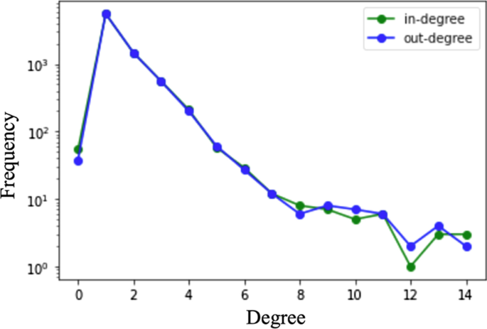
In this multilayered network, we can examine the kind of degree distribution we have, shown in Fig. 6. We can see a high tendency of having both the in-degree and out-degree equal to one (part of a line) and two to four (stations that have intersections of lines of one or more modes). We can also see some nodes with an out-degree of 0. These are start and end stations, respectively, that have no reciprocal edges in the opposite direction. Stations with in-degree and out-degree equal to one can be caused by a significant amount of stations that flow only in one direction, or career end stops have different identifiers depending on orientation. This fact is also explaining the high number of low distances in the figure above. The in-degree is always very close to the out-degree. Since we are looking at a transportation network, this tells us that the majority of the connections between stations flow both ways, forming what is known as a chain (or a line), even though there are apparent exceptions (stations that connect with many stations) as we can see on the tail of the plot with a log scale.

Fig. 6

Degree distribution of the multimodal transport network

4.4 How many stops do we have on average between each station?

To answer this question, we look at the average path length in the number of stops between two stations (not the length of the path itself). For the largest mutually connected component, the average path length (APL) is about 34.6878. This means that, on average, to get from a station/stop to any other on the network, we have to go through about 35 stations/stops before reaching the destination (this number includes multimodal travels as well). Per layer, this value is usually smaller (METRO: 7.7176, CP: 10.2072, FERTAGUS: 5.0, CARRIS: 25.8734, RODLISBOA: 36.9525, SULFERTAGUS: 34.7543, TRANSTEJO: 1.5, TST: 43.3558). However, each layer covers a smaller area than the composition of all the layers. In the case of TST, the APL is higher than in the composition of all the layers. This means that multimodality can be helpful in avoiding many stops.

4.5 Which stations connect travelers from different parts of the city?

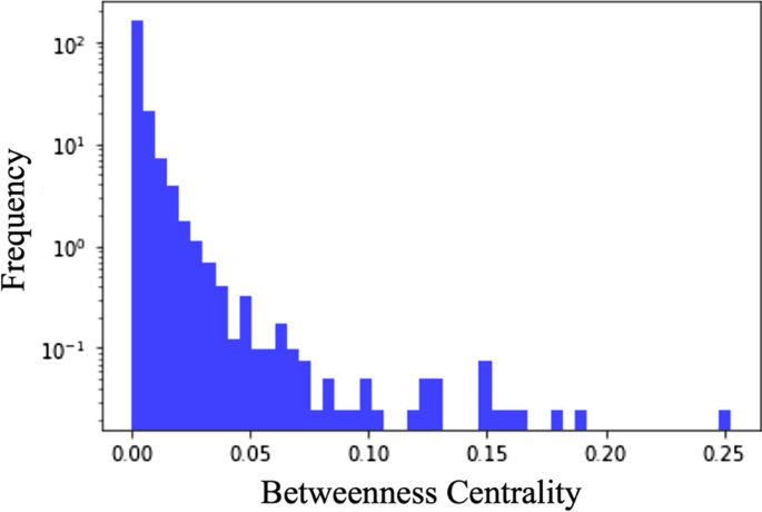
In the case of transportation networks, it is interesting to measure the betweenness centrality to understand which nodes connect different communities of stations, i.e., sets of interconnected stations within a region. In the multilayer network, we identify some stations that have a very high centrality (See Fig. 7). These are mainly from TST. This may be a sign that TST is a kind of bridging layer in some zones. Some examples of such bridging stations are Lisboa Gare do Oriente (0,2529), Setúbal Ciprestes (0,1639), Lisboa Alcântra (0,1592) at TST. METRO also has three stations with exceptionally high betweenness centrality, including Campo Grande (0,1813), Oriente (0,1504), and Cidade Unversitária (0,1480). Rod Lisboa also has a station with a very high betweenness centrality, Lisboa Campo Grande (0,1879). With this simple analysis, we can see that both Lisboa Campo Grande and Lisboa Oriente are multimodality hubs that bridge across different layers.

Fig. 7

Betweenness centrality distribution: In the graph, we can clearly see a few nodes with very high centrality. These are the nodes that represent the stations mentioned above

The left skew on the betweenness centrality may indicate the same type of distribution on node criticality since the betweenness centrality on the node measures the number of shortest paths that include that node. So these results are similar to the ones found in the literature [12].

4.6 Are the central stations directly connected with one another?

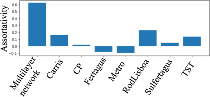
To understand the role of degree-degree correlations, we look at degree assortativity to understand if central stations are connected to one another. This measures the similarity of connected nodes concerning their degree. [5] noted that in multilayer networks, degree-degree correlations should be measured system-wide. In that same study, they generalize this concept for these types of networks and apply it to an airport transportation multilayer network. There they also note that the rich-club effect is, in fact, present in such networks, masked due to the high number of peripheral nodes that connect the hubs. However, intralayer, the networks tend to be disassortative as they focus on one specific region.

We observed a similar behavior from Arruda et al. regarding the assortativity, even with the differences, in reality, being represented (air travel versus urban transportation). We calculated the assortativity for the multilayer network and for each layer, observing the same results. In Fig. 8, we see the same pattern described by [5]. We can observe a much higher assortativity in the multilayer network than in any of the single layers. This is reasonably simple to understand since the assortativity is influenced by the high number of multimodal hubs that connect to one another. Analogous to the properties found in past case studies, we may find a kind of a rich-club effect that may not be there because of the many peripheral nodes. This means that between the central stations within the layer, there are less central stations connected to more central stations. Since this is not the focus of this work, it will be left for future studies.

Fig. 8

Assortativity distribution of each layer and the multilayer network

4.7 Impact of different extraction strategies on network connectedness

In this section, we attempt to answer this question by analyzing the behavior of the size of the largest strongly connected component—SCC—over time for the duration of the simulation. Observing Table 3, the most resilient layer is FERTAGUS, and the least resilient layer is RODLISBOA.

Table 3 Normalized AUC across all networks: RB is the most effective node removal strategy in all the networks, with the exception of TRANSTEJO and the multilayer network

Table 3 shows that the RD and RB strategies usually yield the best results across all layers. In other words, this is more often than not the best strategy to measure robustness. Nevertheless, the RB strategy tends to have a faster descent among the different layers, as we can see in Fig. 9. Hence, the failure of intermodal hubs that have a high degree has devastating effects on the multimodal topology. Moreover, the IB and Random strategies seem to have the least impact on the size of the largest SCC. This is expected, and it is a good baseline to understand that the targeting techniques work to measure robustness. There seems to be no strong reason why the ID strategy has a better result than the RD. However, this is the case in SULFERTAGUS, and it should be investigated further. However, the degree is clearly not the targeting metric that yields the most effective stress strategy, so this may be due to the random removal of stations with the same degree and lower betweenness. We postulate that this happens because there may be reasonably large components that have nodes with a high degree; however, removing nodes from these components does not affect the size of the largest component. So, this phenomenon probably has more to do with the metric we are using than the strategy itself. So this means that single-mode networks are more robust targeting in high degree stations. In Fig. 9, we observe that the RD strategy yields a faster decrease. This checks out with the Normalised AUC with the lowest value. In the third graph, we observe that we still need many more edge removals to get the same result of the size of the largest SCC as in node strategies.

Fig. 9

Evolution of SCC size along node extraction strategies for a single layer, CARRIS (left), all layers (middle), and edge removal in multilayer network (right)

4.8 Impact of node and edge targeting on average path length

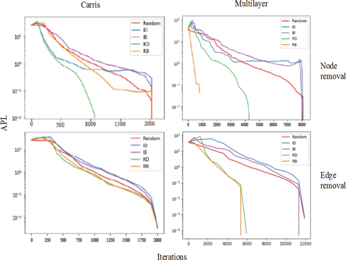
To understand the evolution of path length when targeting stations and pathways, we calculated the APL only for existing paths along with the network. So, if there was no path using the transportation system between two points, this was not accounted for. It is important to note that this strategy may not be the best to measure the robustness of on-road transportation since alternative paths may be available on roads that are not on the usual route. So, we expect the APL to reduce along each time step quickly. We ran the result for each layer and the whole network as well.

Regarding the results for station and pathway targeting of the CARRIS network in Figure 11, the RD is the best strategy. This means that removing the stops with the highest degree has the highest impact on the length of stations one can reach. Note that it may change with alternative routes and redundancy techniques. The remaining strategies have about the same efficiency, with RB being slightly ahead towards the end of the simulation. This result is not unanimous, as we can see in Fig. 10. As we see, RB can either be the best or the worst strategy, depending on the network. This can be due to nodes with high betweenness centrality being part of paths that do not have alternatives. RB providing an efficient strategy indicates lower network robustness. This is the case because it is a topological fragility to have most of the shortest paths within a network going through a single station. In the multimodal network with all the layers (Fig. 11), we see that RB is a strategy that promotes a fast decrease in the APL. This indicates lower network robustness. In the multimodal network, we see that many shortest paths go through the intermodal hubs, allowing parts of the city that have a single mode to be connected with the rest of the city. We can see that the APL decreases much faster in the RB than in the RD for the multilayer, unlike in the CARRIS network. We can also see a slight increase at the beginning of the simulation (only for other extraction strategies). This is due to the removal of less critical stations. The number of removals needed to get the same APL is much higher for edge strategies, meaning node removal is more effective for decreasing APL.

Fig. 10

Evolution of APL along node extraction strategies for METRO (left) and SULFERTAGUS (right)

Fig. 11

Evolution of APL along node (above) and edge (bellow) extraction strategies for the CARRIS and the Multilayer network

4.9 How many nodes or edges do we have to delete to fragment the network into isolated components?

An isolated component is when a node loses all its edges. Since our graph is directed, when we talk about all the edges, we are mentioning both the in and out edges. To be able to answer this question, we used the extraction strategies proposed in the methods and evaluated the evolution of the network by showing the distribution of the isolated components. To accurately understand the extraction strategies, we ran them across every layer in isolation and then in the complete network, except for multimodal hub removal on isolated layers because there are no multimodal hubs in isolated layers. Figure 12 shows the evolution of isolated components for each strategy in the CARRIS layer. In these graphs, we clearly see that RD had the best results. This is the only one that stopped before the end of the simulation because there are only isolated components when it stops. We obtained about the same results in every layer and for multilayer network is also very similar.

Fig. 12

Evolution of the Isolated components (IC) in the CARRIS layer (left) and multimodality network (right) for node removal

We also find that all extraction strategies, except RD, increase and then decrease the number of isolated components (Fig. 12). This means that after we reach the maximum number of ICs, we are only removing isolated nodes. This means that the lower the maximum and the later it is reached, the less effective at measuring the robustness of the isolation of different parts of the city the strategy is. Halfway through RB, we start to see rapid growth. This is because after removing the main bridges from communities, there still are redundancy paths. Once these paths start to be removed, it is simpler to disconnect each community individually. It should be noted that it is likely that a node with a high degree also has a high betweenness centrality since multimodal hubs are often points that connect communities. However, this is not the case since less-connected stations may be essential in connecting different parts of the city. The IB extraction is the worst because we are dividing the problem infinitely. This is virtually dividing the path from A to B into two recursively. In summation, the only effective strategy to measure the vulnerability of disconnecting the network from different parts of the city is RD.

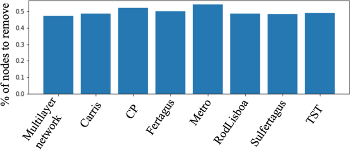
So, to answer the highlighted question in this section, we look at the number of iterations when RD ends the simulation. This is the number of nodes that have been removed when all the remaining nodes are isolated. The higher the percentage of nodes that need to be removed from the total of nodes in this network, the more robust the network is, see Fig. 13. We can see that the robustness across all networks using this metric is about the same.

Fig. 13

Minimum percentage of nodes that need to be removed to separate the network into only isolated components, using targeted extractions. The lower this value, the less resilient this network is

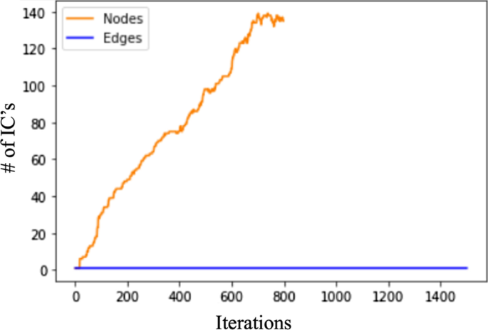
To understand the multimodal hub removal, we recurred to another graph due to scale and purpose. As the graph reaches a pique and then decreases, we can see that we do not need to remove all the multimodal nodes to get isolated layers. As we can see, there is a slight variation when some nodes are removed. This means that removing specific nodes has more impact on the interlayer connections (Fig. 14). We can see that node removal is much better than edge removal, which makes sense since in edges, we only separate in at most 8 ICs (single layers). This is not directly comparable with other strategies, as it only encompasses the removal of about 10% of the nodes. However, from what we can assess, in the beginning, the growth in the number of isolated components follows approximately a linear function, which is slower than RD. However, we can safely conclude that the redundancy of intermodal hubs is the best way to ensure connectedness in this multimodal network since not all layers are redundant in all areas of the city. Redundancy in all areas of the city would be much more costly and may even cause other issues like consuming space of the already established routes.

Fig. 14

Evolution of the Isolated components using the Multimodal Hubs removal strategy

On the other hand, there are edge extractions. In this case, it is expected that we have to remove all the edges to have all nodes isolated; Fig. 15 shows precisely that. The behavior of extraction per layer and in the multilayer network is identical, as can be seen in both graphs in Fig. 15. Contrary to node targeting, the worst strategy is RD, and the best strategy is IB. The RD is always the worst strategy. This is the case because we are removing edges from nodes with high degrees. We can conclude that the betweenness centrality is an adequate metric for edge targeting and degree is better for node targeting. This means that removing single pathways that are in many shortest paths has a higher impact than removing single pathways that lead to high degree stations. However, deactivation or failure of high degree stations has the highest impact. High degree stations are the ones that are usually more central geographically and have a more critical role in connecting different modes of transport.

Fig. 15

Evolution of Isolated components along edge extraction strategies for CARRIS (left) and for the multilayer network (right)

4.9.1 Impact of removing nodes versus edges

We found that node extractions are more efficient than extracting the edges, as we need more removals to get the same increase of ICs and decrease of APL and decrease of SCC. This means that removing the high degree stations has a much higher impact than removing every single pathway that leads to each important station individually. As previous Figures indicate, it takes much more iterations to disconnect a network by extracting the edges. This happens for various reasons. Expectedly, there are more edges than nodes, so more iterations are needed to create the same impact. Another important reason is that when we remove a node, we also remove all the edges of that specific node, and the contrary is not the case. This happens because an incident in a pathway to a station may not impact the station, and an incident on a station may more probably impact the pathways through it. This makes the node removal more damaging to the network.

On the SCC and the APL evaluation, we also see that edges’ extractions are very similar to each other and also less efficient at disconnecting the network than nodes removal. We can conclude that the network has various redundant paths. Hence, by removing edges, we can go to the same destination by going through more stations.

It is also important to note that in the IC evaluation, the ID and RD removal extractions on the edges are not as efficient as in the nodes and have a slow impact. With a slow impact, we mean that we need to remove more edges to create the same damage as the node removal. This happens because, when we base the extraction on the edge degree, we are extracting edges of hub nodes (nodes with high degrees). This means that we are removing edges from nodes with lots of edges and so it does not show the effect at first.

4.9.2 Should we recalculate the degree and betweenness after each extraction?

Often, the random strategy is better than the strategies which do not recalculate the new metrics of the new graph (IB and ID). On the other hand, RB and RD removal strategies can be very effective (Table 3) yet not so computationally efficient. They take much more computational power to compute metrics, especially the RB. As can be seen in previous sections, recalculating degree after each node removal has proven to be beneficial, but recalculating betweenness centrality has yielded relatively stable results for ICs and wildly variable results in APL evolution. Intuitively this could probably be explained by the lack of redundant paths in some networks, which is a fair way to assess its robustness. Both RB and RD strategies have the same similar results across layers and are the best ones to reduce the SSC.

For the edge removing strategies, in the case of the goal being generating more isolated components, recalculating the betweenness centrality yields the worst results. These results are curious as they are quite different from the ones proposed by [22]:1), “suggesting that the network structure changes as important vertices or edges are removed.”

Despite the RD and RB strategy overall having better results for node extractions, in massive graphs seems unfeasible to calculate the betweenness centrality per each iteration. Another possible strategy is, instead of calculating per each iteration, i.e., each node removal, to calculate this metric per each percentage of removals. In this way, we are avoiding the complexity with the trade-off of slightly disrupting the result. This is a suboptimal solution; however, it is shown to be viable to the extent of the empirical results.

4.9.3 What is the impact of cascading failures?

The cascading failures are a complex topic, and we have only scratched the surface. On cascading failures, we used two removal strategies: entirely deleting a transportation line (e.g., route) and removing the neighbors of a given node (e.g., station). For the first removal, we simulated the crash of each line separately, that is, one line at a time, and measured the number of ICs, then repeated the process for each line after resetting the network to its initial condition. We were able to get the maximum number of 6 separated components from a single line by doing this assessment. This line/route connects Pontinha and Campo Grande, operated by RodLisboa (bus road operator). It is mainly a commuting route that connects passengers living in Pontinha (county within LMA) with Lisbon city, mainly for home-to-work purposes.

In our second simulation, we applied the failure removal approach of a neighbor. Line Failure was used as a model for the simulation. We estimated the neighbors of each node, eliminated them, and gathered the metric of the isolated component. We chose three layers of a node’s neighbors since the average number was closer to the average number of each line when comparing the two. Odivelas was discovered to be the key point in this method, with a maximum number of isolated components of 10.

We can see that the nodes that connect Lisbon city with other counties within LMA are critical to the organization of the city’s public transportation system. Nonetheless, this Neighbour Failure technique has much more devastating effects than the Line Failure strategy, with nearly double the network damage (6 vs. 10), but this is based on a small sample. These results tell us that the impact of a localized failure that deactivates that spot in several layers has a higher impact than a line failure in this topology. However, this result may vary depending on the region since localized failures in remote areas have a lower relative impact.

5 Conclusions and future works

In this work, we propose a measurement method of the topological robustness of a multimodal network by using different network analysis metrics and by performing node and edge percolation with specific criteria. Then we proceed to apply these measurements to the Lisbon Metropolitan Area Multimodal network, to further understand applicability. We modeled and analyzed the structure of Lisbon’s public transport network to measure its robustness according to a multimodal stance. Results allow us to understand the geographic information inherent to the multiplex network by programming a 3D plotting method. After calculating and interpreting some of the network metrics, results indicate that multimodal coordination can help diminish the number of stops in a pathway. After identifying stations that work as bridges between different layers and communities, we then analyzed different extraction strategies based on previous work. This is an important step to guide the assessment of classic robustness metrics in the context of multimodal transport networks. The target metrics include the size of the largest SCC (strongly connected components), APL (average path length), and ICs (isolated components), as well as a proposed normalized AUC (area under the curve). Hence, we observed that the selection of metrics should be constrained to the goal and type of removal (edge vs. node).

Results show that the strategies that depend on recalculating metrics are generally more effective, with the exception of a particular case of edge removal using betweenness centrality to maximize ICs, which counter-intuitively had better results for the IB (initial betweenness) strategy. Even though we were able to postulate on this phenomenon, further research needs to be done to understand it. We also showed that the resilience tests needed to remove about half the nodes of the network to leave all the remaining nodes wholly disconnected. This is a phenomenon that happens in all layers and the multilayer network as well, suggesting that betweenness targeting is the best way to measure robustness across the different strategies. We also verified higher assortativity phenomena in multilayered networks, in contrast to single layers, highlighting the importance of intermodal hub redundancy.

Based on the robustness tests, we were able to conclude that the most effective method for targeting nodes is RD (recalculate degree). However, in some cases, RB (recalculate betweenness) yielded better results for multilayer APL decadence (both for nodes and edges strategies), although it showed higher variability. This means that the number of pathways to a station is less important than how many shortest paths go through that station in a multimodal scenario when completely disconnecting the network. For decreasing the size of the largest SCC, RD yielded better results for the multilayer network. However, for most of its individual layers, the best strategy was actually RB. This means that to divide a multimodal network into disconnected regions, high degree station failures have a higher impact than high betweenness station failures. However, to yield the same result in a single-mode network, betweenness is a more relevant metric, highlighting the impact of the network topology as the vulnerabilities linked to a multimodal network considerably differ from a single-layer network.

With the normalized AUC, we were able to compare, side by side, the robustness of each transport operator-specific network, regardless of its size. Carris, RodLisboa, SulFertagus, and TST show inferior robustness to the remaining networks. The two most robust networks were Fertagus and Transtejo. Nevertheless, this result may be due to inflation on smaller sizes, pinpointing the need for non-uniform scaling factors for the AUC normalization. The multilayer network was more resilient than one-half of the layers but less than the other. We also performed cascading failures in the network to understand some of the expected impacts. Still, since it is a vast and exciting topic, we focused on two major strategies. We showed that neighbor failure is more effective than line failure in this particular network, even though they are moderately similar in the structure of the present network. The impact yield from different cascading events can be the subject of a future study. For example, instead of simulating random line crashes, using simulated failures on more than one line at a time and using a specific measure would be more effective in determining which lines are more critical, like what we have done with the degree and betweenness centrality targeting. The second elimination could be investigated further by experimenting with more layers of neighbors. The archetype of these might be a combination of these two strategies, attempting to fail lines that are close to other lines using information from each node’s neighbors. We also identified that further research is needed on the effect of the rich club on peripheral nodes on robustness and cascading effects in the context of this network. Last but not least, we recognize the importance of the analysis of the capacity, ridership and bottlenecks. Nevetheless, topological views also yield interesting results. More specifically, the gathered results in this study suggest that robustness can be objectively measured using network metrics and percolation simulations. The impact of such simulations can be compared regardless of the network size or structure in any multimodal transportation scenario. Moreover, research findings point out that we can use the targeting techniques to understand network recoverability (resilience stance) by focusing on stations with hub characteristics (higher centrality) or high betweenness. This study allows practitioners and urban transportation policymakers to tackle the impact of negative disruption in multimodal transportation networks.

References

Al-Deek, H., & Emam, E. B. (2006). New methodology for estimating reliability in transportation networks with degraded link capacities. Journal of Intelligent Transportation Systems, 10(3), 117–129.
Aleta, A., Meloni, S., & Moreno, Y. (2017). A multilayer perspective for the analysis of urban transportation systems. Scientific Reports, 7, 44359.
Aparicio, J. T., Arsenio, E., & Henriques, R. (2021). Understanding the Impacts of the COVID-19 pandemic on public transportation travel patterns in the city of Lisbon. Sustainability, 13(15), 8342.
Aparicio, J. T., Trinca, M., Castro, D., Henriques, R. (2021b). “Vehicle Smart Grid Allocation Using Multi-Agent Systems Sensitive to Irrational Behavior and Unstable Power Supply.” Pp. 1–6 in (2021b) 16th Iberian Conference on Information Systems and Technologies (CISTI).
de Arruda, G., Ferraz, E. C., Moreno, Y., & Rodrigues, F. A. (2016). On degree-degree correlations in multilayer networks. Physica D: Nonlinear Phenomena, 323, 5–11.
Bernardo, M. R., Neto, M. D. C., de Lisboa, N., Aparicio, M., de Lisboa. (2019). “Smart Mobility: A Multimodal Services Study in the Metropolitan Area of Lisbon.” Smart Mobility 20.
Bocewicz, G. (2014). “Robustness of multimodal transportation networks.” Eksploatacja i Niezawodność 16.
Bogart, D. (2009). Inter-modal network externalities and transport development: evidence from roads, canals, and ports during the english industrial revolution. Networks and Spatial Economics, 9(3), 309–338.
Brandes, U. (2001). A faster algorithm for betweenness centrality. Journal of Mathematical Sociology, 25(2), 163–177.
Campbell, A. M., & Van Woensel, T. (2019). Special issue on recent advances in urban transport and logistics through optimization and analytics. Transportation Science, 53(1), 1–5. https://doi.org/10.1287/trsc.2018.0882
Cats, O., & Jenelius, E. (2018). Beyond a complete failure: The impact of partial capacity degradation on public transport network vulnerability. Transportmetrica B: Transport Dynamics, 6(2), 77–96.
Cats, O., Koppenol, G.-J., & Warnier, M. (2017). Robustness assessment of link capacity reduction for complex networks: Application for public transport systems. Reliability Engineering & System Safety, 167, 544–553.
Chen, A., Yang, H., Lo, H. K., & Tang, W. H. (2002). Capacity reliability of a road network: An assessment methodology and numerical results. Transportation Research Part B: Methodological, 36(3), 225–252.
Clark-Ginsberg, A. (2016). “What’s the Difference between Reliability and Resilience.” Department of Homeland Security. March.
Clifton, K., & Muhs, C. D. (2012). Capturing and representing multimodal trips in travel surveys: review of the practice. Transportation Research Record, 2285(1), 74–83.
Derudder, B., Liu, X., Kunaka, C., & Roberts, M. (2014). The connectivity of south asian cities in infrastructure networks. Journal of Maps, 10(1), 47–52.
Ding, R., Ujang N., bin Hamid, H., Abd Manan, M. S, He, Y, Li, R., Wu, J. (2018). “Detecting the urban traffic network structure dynamics through the growth and analysis of multi-layer networks.” Physica A: Statistical Mechanics and Its Applications 503:800–817
Du, W.-B., Zhou, X.-L., Lordan, O., Wang, Z., Zhao, C., & Zhu, Y.-B. (2016). Analysis of the chinese airline network as multi-layer networks. Transportation Research Part E: Logistics and Transportation Review, 89, 108–116.
Elvas, L. B., Mataloto, B. M., Martins, A. L., & Ferreira, J. C. (2021). Disaster management in smart cities. Smart Cities, 4(2), 819–839.
Fernandes, N., Moro, S., Costa, C. J., & Aparício, M. (2020). Factors influencing charter flight departure delay. Research in Transportation Business & Management, 34, 100413. https://doi.org/10.1016/j.rtbm.2019.100413
Heinen, E., & Mattioli, G. (2019). Multimodality and CO2 emissions: A relationship moderated by distance. Transportation Research Part D: Transport and Environment, 75, 179–196.
Holme, P., Kim, B. J., Yoon, C. N., & Han, S. K. (2002). Attack vulnerability of complex networks. Physical Review E, 65(5), 056109.
Immers, B., Yperman, I., Stada J., Bleukx, A. (2002). “Reliability and Robustness of Transportation Networks.” Problem Survey and Examples.
INE, I. P. (2018). Mobilidade e Funcionalidade Do Território Nas Áreas Metropolitanas Do Porto e de Lisboa 2017. Instituto Nacional de Estatística, I. P. Av.António José de Almeida,1000–043 Lisboa, Portugal: Instituto Nacional de Estatística, I. P.
Klau, G. W., & Weiskircher, R. (2005). Robustness and resilience. In U. Brandes & T. Erlebach (Eds.), Network analysis (pp. 417–437). Berlin: Springer. https://doi.org/10.1007/978-3-540-31955-9_15
Kouvelis, P., Gang, Y. (2013). Robust Discrete Optimization and Its Applications. Vol. 14. Springer Science & Business Media.
Liu, R., Chen, Y., Jianping, Wu., Tingbao, Xu., Gao, L., & Zhao, X. (2018). Mapping spatial accessibility of public transportation network in an urban area–a case study of shanghai Hongqiao transportation hub. Transportation Research Part D: Transport and Environment, 59, 478–495.
Lu, H., Wang, J., & Zhang, P. (2004). Urban transport structure optimization based on energy consumption. Journal-Tsinghua University, 44(3), 383–386.
Masel, J., & Siegal, M. L. (2009). Robustness: Mechanisms and consequences. Trends in Genetics, 25(9), 395–403.
Migliore, M., & Catalano, M. (2007). “Urban public transport optimization by bus ways: a neural network-based methodology”. Urban transport xiii–urban transport and the environment in the 21st century. Book Series: WIT Transactions on the Built Environment, 96, 347–356.
Montes-Orozco, E., Mora-Gutiérrez, R. A., Obregón-Quintana, B., de-los-Cobos-Silva, SG., Rincón-García, EA., Lara-Velázquez, P., Gutiérrez-Andrade, MA. (2020). “Inverse Percolation to Quantify Robustness in Multiplex Networks.” Complexity 2020.
Ramos, C., Zêzere, J. L., & Reis, E. (2010). “Avaliação Da Susceptibilidade Aos Perigos Naturais Da Região de Lisboa e Vale Do Tejo”. Prospectiva e Planeamento. Ordenamento Territorial e Sustentabilidade, 17, 57–73.
Scott, D. M., Novak, D. C., Aultman-Hall, L., & Guo, F. (2006). Network robustness index: A new method for identifying critical links and evaluating the performance of transportation networks. Journal of Transport Geography, 14(3), 215–227.
Stamos, I., Mitsakis, E., Salanova, J. M., & Aifadopoulou, G. (2015). Impact assessment of extreme weather events on transport networks: A Data-driven approach. Transportation Research Part D: Transport and Environment, 34, 168–178.
Sullivan, J. L., Novak, D. C., Aultman-Hall, L., & Scott, D. M. (2010). Identifying critical road segments and measuring system-wide robustness in transportation networks with isolating links: A link-based capacity-reduction approach. Transportation Research Part A: Policy and Practice, 44(5), 323–336.
Tavasszy, L., Minderhoud, M., Perrin, J.-F., & Notteboom, T. (2011). A Strategic network choice model for global container flows: Specification, estimation and application. Journal of Transport Geography, 19(6), 1163–1172.
UN. (2018). “World Urbanization Prospects.”
Varga, I. (2016). Weighted multiplex network of air transportation. The European Physical Journal B, 89(6), 139.
Zhang, H., Cui, H., Wang, W., & Song, W. (2020). Properties of Chinese railway network: Multilayer structures based on timetable data. Physica A: Statistical Mechanics and Its Applications, 560, 125184.
Zhang, X., Miller-Hooks, E., & Denny, K. (2015). Assessing the role of network topology in transportation network resilience. Journal of Transport Geography, 46, 35–45.
Zhou, Di., Eugene Stanley, H., D’Agostino, G., & Scala, A. (2012). Assortativity decreases the robustness of interdependent networks. Physical Review E, 86(6), 066103.
Zhou, Y., & Wang, J. (2017). Critical link analysis for urban transportation systems. IEEE Transactions on Intelligent Transportation Systems, 19(2), 402–415.
Acknowledgements
We thank Daniel Castro and Miguel Trinca for their contributions regarding the code and insightful discussions along with Professor Francisco C. Santos for the proposed challenge. We also thank CARRIS, METRO and Câmara Municipal de Lisboa (Gabinete de Mobilidade and Centro de Operações Integrado) for the provision of data, support, and valuable feedback. This work was further supported by national funds through Fundação para a Ciência e Tecnologia (FCT) under project ILU (DSAIPA/DS/0111/2018) and INESC-ID pluriannual (UIDB/50021/2020).
Funding
This work is further supported by national funds through Fundação para a Ciência e Tecnologia under project ILU—Integrative Learning from Urban Data and Situational Context for City Mobility Optimization (DSAIPA/DS/0111/2018) and INESC-ID pluriannual (UIDB/50021/2020).
Author information
Authors and Affiliations
Contributions
All authors (JTA, EA, RH) contributed to the research study. JTA conducted the simulation and data analysis, and prepared the first version of the manuscript. EA and RH carried out the research supervision and validation of the use case. RH was responsible for the project administration. All authors (JTA, EA, RH) approved the final manuscript.
Corresponding author
Ethics declarations
Competing interests
The authors declare that they have no competing interest.
Additional information
Publisher's Note
Springer Nature remains neutral with regard to jurisdictional claims in published maps and institutional affiliations.
Rights and permissions
Open Access This article is licensed under a Creative Commons Attribution 4.0 International License, which permits use, sharing, adaptation, distribution and reproduction in any medium or format, as long as you give appropriate credit to the original author(s) and the source, provide a link to the Creative Commons licence, and indicate if changes were made. The images or other third party material in this article are included in the article's Creative Commons licence, unless indicated otherwise in a credit line to the material. If material is not included in the article's Creative Commons licence and your intended use is not permitted by statutory regulation or exceeds the permitted use, you will need to obtain permission directly from the copyright holder. To view a copy of this licence, visit http://creativecommons.org/licenses/by/4.0/.
About this article
Cite this article
Aparicio, J.T., Arsenio, E. & Henriques, R. Assessing robustness in multimodal transportation systems: a case study in Lisbon. Eur. Transp. Res. Rev. 14, 28 (2022). https://doi.org/10.1186/s12544-022-00552-3
Received:
Accepted:
Published:
DOI: https://doi.org/10.1186/s12544-022-00552-3